Presented by Eric Wells
Eric Wells is the author of Developing Microsoft Excel 5 Solutions, a book on advanced Excel/VBA development published by Microsoft Press. Eric has been with Microsoft since July of 1992. He worked for two years as the product manager for Microsoft® Excel, directing the marketing rollout of Visual Basic® for Applications (VBA) in Excel 5. Eric has lectured on developing with Excel and VBA at numerous conferences throughout the United States and Europe. Eric is currently the product manager for Microsoft Office and host of the Microsoft Office Solutions show on Microsoft Television. Eric can be reached over the Internet at ericwell@microsoft.com.
Much of the material in this paper is covered in detail in Developing Microsoft Excel 5 Solutions (ISBN 1-55615-684-7) published by Microsoft Press.
Sample files for this session include:
All macros in this document are included in the xl301.xls file. Load all files into a common directory on your hard drive. In order to run the VBA macros in xl301.xls, you must set up an Access 2 ODBC data source that points to the saledata.mdb file. Name this data source "saledata".
The xl301.xls workbook contains macros that make reference to the SQL functions in xlodbc.xla. To run these functions, you must have copies of xlodbc.xla and xlodbc.dll on your hard drive as well—copy the versions of these files from your session files diskette/CD into the same directory as xl301.xls.
The PivotTable object is one of the most advanced objects in Microsoft Excel. PivotTables provide a tool that allows users to view data from either an external database or an Excel worksheet database in various different dynamic views. The versatility of the pivottable provides a powerful interface for summarizing and interpreting large amounts of database data.
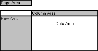
The pivottable object is segmented into four main areas:
Graphically, the four areas of the pivottable appear as follows:

Building a pivottable involves reading a data set into an internal RAM memory cache and then specifying which columns of the data set will go into each of the four areas of the pivottable—row, column, data and page areas. Two things are important to note about assigning different data set columns to the different areas of the pivottable: first, it is possible to assign multiple columns to each area of the pivottable; second, if a data set column is assigned to the row, column or page areas of the pivottable, then only the unique values of that particular dataset column will be displayed in the pivottable—that is the data in the data area of the pivottable will be summarized according to items displayed in the row, column and page areas.
The pivottable object actually contains an OLE object hierarchy in its own right. There are three levels of programmable objects in the pivottable hierarchy:
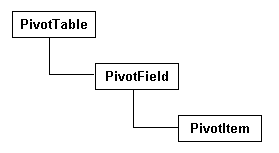
The PivotTable object is used to reference the pivottable itself. The PivotField object is used to reference the different data set columns which are placed in the row, column, data and page areas of the pivottable. The PivotItem object is used to reference the unique values that exist in a pivotfield—PivotItem is therefore, really only of use in working with unique items in pivotfields in the row, column or page areas of a pivottable.
Because the data behind a pivottable is stored in a RAM memory cache, manipulation of the data within a pivottable is generally accomplished at a very high level of performance. It is possible for a user to move a pivotfield from one area of the pivottable to another—say from the page area to the row or column area. With data stored in RAM, Excel can quickly perform the operation of re-architecting the pivottable to meet the new configuration as specified by the user.
One may question when in an Excel application it is necessary to programmatically create a pivottable. In reality, there are few instances where such programmatic creation of a pivottable is necessary or even practical. However, it is quite useful in some applications to "rebuild" an existing pivottable based on certain conditions. We, therefore, are going to look at the process of programmatically creating a pivottable first, and then extend the discussion to cover instances in applications where it is useful to re-build a pivottable.
A pivottable is programmatically created through calling the PivotTableWizard method of the Worksheet object. The PivotTableWizard method takes the following arguments:
SourceType: One of four values indicating the source of the pivottable data:
SourceData: The actual source of the data. Values passed for SourceData will differ depending on the value passed for sourcetype:
TableDestination: A worksheet range where the resulting pivottable will reside.
TableName: A string to be assigned as the name of the pivottable.
RowGrand: True/False—if True, then grand totals will be displayed for each row in the pivottable.
ColumnGrand: True/False—if True, then grand totals will be displayed for each column in the pivottable.
SaveData: True/False—if True, then pivottable cache data is saved with the pivottable when the workbook file containing the pivottable is saved to disk.
HasAutoFormat: True/False—if True, then any autoformats applied to the pivottable will be saved with the pivottable—and such autoformats will "stick" with the pivottable no matter what shape or size the pivottable takes on.
AutoPage: True/False—valid only if the sourcetype argument is True. If True, Excel creates a pagefield for the consolidation.
Let's take a look at a macro that can be used to create a pivottable programmatically. The example below as well as the rest of the pivottable examples in this paper are based off of an external Access 2 database named saledata.mdb and represented by an ODBC data source named "saledata".
Sub Mod1CreatePivot1()
    Dim SQLString As String
    Dim PivotSheet As Worksheet
    Set PivotSheet = Worksheets("PivotSheet")
    SQLString = "Select * FROM Revenue"
    PivotSheet.PivotTableWizard _
        SourceType:=xlExternal, _
        SourceData:=Array("DSN=SaleData", SQLString), _
        TableDestination:=PivotSheet.Range("B5"), _
        TableName:="Pivot1"
End Sub
When you run CreatePivot1 above, the resulting worksheet appears as follows:
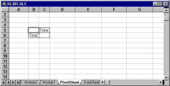
Calling the PivotTableWizard method in CreatePivot1 above only served to read the data set into the internal RAM memory cache and allocate space on the worksheet for the pivottable. The macro gave no instructions to Excel on which areas of the table to place which pivotfields. To actually build the pivottable, then, you must specify where to place the pivotfields that make up the data set—this is done by setting the Orientation property of the PivotField object. Before we get to that, let's take a quick look at a simple macro that we will use to delete all pivottables on a worksheet. Macro DeletePivotTables below uses a For-Each-Next loop on the pivottables collection on PivotSheet worksheet to call the Clear method on TableRange2 of each pivottable on the worksheet—this will effectively, delete each pivottable that exists on the first worksheet:
Sub Mod1DeletePivotTables()
    Dim x As Variant
    For Each x In Worksheets("PivotSheet").PivotTables
        x.TableRange2.Clear
    Next
End Sub
Okay, back to setting the Orientation property of the PivotField object. Orientation can take on one of four values corresponding to the four areas of the pivottable: xlRowField, xlColumnField, xlDataField and xlPageField. Let's now take a look at a macro that will build a pivottable and actually place different pivotfields into the different areas of the pivottable:
Sub Mod1CreatePivot2()
    Dim Pivot1 As PivotTable
    Dim SQLString As String
    Dim PivotSheet As Worksheet
    Set PivotSheet = Worksheets("PivotSheet")
    Mod1DeletePivotTables
    SQLString = "Select * From Revenue"
    Set Pivot1 = PivotSheet.PivotTableWizard _
        (SourceType:=xlExternal, _
        SourceData:=Array("DSN=SaleData", SQLString), _
        TableDestination:=PivotSheet.Range("B5"), _
        TableName:="Pivot1")
    With Pivot1
        .PivotFields("Region").Orientation = xlPageField
        .PivotFields("Period").Orientation = xlRowField
        .PivotFields("Category").Orientation = xlColumnField
        .PivotFields("Revenue").Orientation = xlDataField
    End With
End Sub
The resulting pivottable from CreatePivot2 above appears as follows:
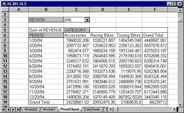
CreatePivot2 has resulted in the creation of what appears to be much more like a pivottable. Moving forward, there may be additional formatting or various other options that we may wish to implement on the pivottable. CreatePivot3 below builds the same pivottable as CreatePivot2 above, however, in this case, the Revenue pivotfield in the data area is formatted with a currency format, and one of Excel's built-in autoformats is applied to the table—xlClassic3 in this case.
Sub Mod1CreatePivot3()
    Dim Pivot1 As PivotTable
    Dim SQLString As String
    Dim PivotSheet As Worksheet
    Set PivotSheet = Worksheets("PivotSheet")
    Mod1DeletePivotTables
    SQLString = "Select * From Revenue"
    Set Pivot1 = PivotSheet.PivotTableWizard _
        (SourceType:=xlExternal, _
        SourceData:=Array("DSN=SaleData", SQLString), _
        TableDestination:=PivotSheet.Range("B5"), _
        TableName:="Pivot1")
    With Pivot1
        .PivotFields("Region").Orientation = xlPageField
        .PivotFields("Period").Orientation = xlRowField
        .PivotFields("Category").Orientation = xlColumnField
        With .PivotFields("Revenue")
            .Orientation = xlDataField
            .NumberFormat = "$#,##0_);($#,##0)"
            .Name = "Rev"
        End With
        .TableRange2.AutoFormat format:=xlClassic3
    End With
End Sub
There are certain situations where it is not practical to bring an entire database table into the pivottable RAM cache. When dealing with large datasets in a pivottable RAM cache, the main performance drain comes in the initial population of the cache, as well as any refreshing of the cache that is done (by calling the RefreshTable method on the pivottable object). To avoid any major negative impact on performance that might come with the initial population or refresh of a pivottable cache, it may be desirable to bring only a portion of a database table into the pivottable cache. When working with external data sources, this can be accomplished through manipulation of the SQL string that is passed as part of the source data argument for the pivottablewizard method. In the macros above, we used the pivottablewizard method to bring an entire database table into the RAM cache—the Revenue table. Let's assume that the Revenue table actually contains tens of thousands of records and that bringing the entire table into the RAM cache results in an unacceptable drain on performance. It may be more feasible to bring in only a portion of the data—say for the "West" region only. To do this, we change the SQL statement to the following:
Select * From Revenue WHERE Region Like 'West'
Macro CreatePivot4 builds a pivottable that contains data for the West region only:
Sub Mod1CreatePivot4()
    Dim Pivot1 As PivotTable
    Dim SQLString As String
    Dim PivotSheet As Worksheet
    Set PivotSheet = Worksheets("PivotSheet")
    Mod1DeletePivotTables
    SQLString = "Select * From Revenue WHERE Region Like 'West'"
    Set Pivot1 = PivotSheet.PivotTableWizard _
        (SourceType:=xlExternal, _
        SourceData:=Array("DSN=SaleData", SQLString), _
        TableDestination:=PivotSheet.Range("B5"), _
        TableName:="Pivot1")
    With Pivot1
        .PivotFields("Region").Orientation = xlPageField
        .PivotFields("Period").Orientation = xlRowField
        .PivotFields("Category").Orientation = xlColumnField
        With .PivotFields("Revenue")
            .Orientation = xlDataField
            .NumberFormat = "$#,##0_);($#,##0)"
            .Name = "Rev"
        End With
        .TableRange2.AutoFormat format:=xlClassic3
    End With
End Sub
By altering the SQL statement as we have done in CreatePivot4 above, we can greatly reduce the amount of time that is required to populate the pivottable cache. However, there is one glaring flaw in the pivottable that is created with CreatePivot4 above—there are only two items in the pagefield dropdown—"West" and "(All)"—choosing either will display data for only the West region. With this pivottable, how would a user be able to choose to view data for one of the other regions? With the current structure there is no way—and essentially, it doesn't make a whole lot of sense to have a pagefield dropdown with two items that cause the pivottable to display the same thing. So before we go on, let's first build the pivottable again—but this time without the pagefield dropdown:
Sub Mod1CreatePivot5()
    Dim Pivot1 As PivotTable
    Dim SQLString As String
    Dim PivotSheet As Worksheet
    Set PivotSheet = Worksheets("PivotSheet")
    Mod1DeletePivotTables
    SQLString = "Select * From Revenue WHERE Region Like 'West'"
    Set Pivot1 = PivotSheet.PivotTableWizard _
        (SourceType:=xlExternal, _
        SourceData:=Array("DSN=SaleData", SQLString), _
        TableDestination:=PivotSheet.Range("B5"), _
        TableName:="Pivot1", _
        SaveData:=False)
    With Pivot1
        .PivotFields("Period").Orientation = xlRowField
        .PivotFields("Category").Orientation = xlColumnField
        With .PivotFields("Revenue")
            .Orientation = xlDataField
            .NumberFormat = "$#,##0_);($#,##0)"
            .Name = "Rev"
        End With
        .TableRange2.AutoFormat format:=xlClassic3
    End With
End Sub
You will notice that in CreatePivot5 above, we've added an additional argument for the pivottablewizard method—False has been passed for SaveData. Passing False for SaveData results in the pivottable cache not being saved with the workbook file when the file is saved to disk. If False is passed for SaveData, then if the file is saved, closed and then reopened, no data will exist in the pivottable cache—attempts to use the pivottable will fail under such circumstances. While setting SaveData to False will result in smaller file size (due to no pivottable cache being saved with the file), you must be certain to automatically refresh the cache when the file is opened—this can be accomplished through use of an auto_open macro that includes the following statement:
Worksheets("PivotSheet").PivotTables("Pivot1").RefreshTable
Next, let's add a DropDown object to the worksheet containing the pivottable. We want the dropdown object to contain a listing of all of the unique items in the Region field in the Revenue table. The best way to obtain the unique items is to issue a SQLRequest command and pass the following SQL statement (this statement will also order the return items):
Select Distinct Region From Revenue Order by Region
The AddRegionDropDown macro below will actually add a dropdown object to the worksheet containing the pivottable and initialize it with unique values from the Region column of the Revenue table in the external database. It is possible to add a dropdown to a worksheet manually, by using the dropdown tool on the forms toolbar—but in this case, we'll go ahead and add one programmatically:
Sub Mod1AddRegionDropDown()
    Dim SQLString As String
    Dim PivotSheet As Worksheet
    Dim Drop1 As DropDown
    Dim x As Integer
    Set PivotSheet = Worksheets("PivotSheet")
    SQLString = "Select Distinct Region " & _
                "From Revenue Order by Region"
    PivotSheet.DropDowns.Add(49, 20, 90, 10).Name = "Drop1"
    Set Drop1 = PivotSheet.DropDowns("Drop1")
    PivotSheet.Select
    With Drop1
        .List = SQLRequest("DSN=SaleData", SQLString)
        .Placement = xlFreeFloating
        .OnAction = "Mod1ChangeRegion1"
        For x = 1 To .ListCount
            If .List(x) = "West" Then
                .Value = x
                Exit For
            End If
        Next
    End With
End Sub
After adding the dropdown to the worksheet, the pivottable and dropdown together appear as follows:
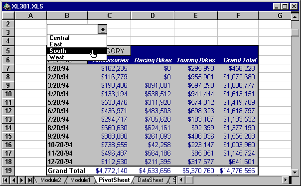
Macro ChangeRegion1 below builds a SQL string based on the item selected from dropdown Drop1 on the PivotSheet worksheet—this SQL string is then passed to the pivottablewizard method to refresh the pivottable cache with a new data set. A couple of things to note: first, we are not actually deleting and then re-building the pivottable here—instead, we are merely calling the pivottablewizard method on an existing pivottable; second, before we can call the pivottablewizard method on an existing table, we must first select the worksheet containing the pivottable and then select a range within the pivottable—in this case, tablerange2 as been selected (tablerange2 encompasses the entire range that is occupied by all areas of the pivottable):
Sub Mod1ChangeRegion1()
    Dim PivotSheet As Worksheet
    Dim Drop1 As DropDown
    Dim Pivot1 As PivotTable
    Dim RegionName As String
    Dim SQLString As String
    Set PivotSheet = Worksheets("PivotSheet")
    Set Pivot1 = PivotSheet.PivotTables("Pivot1")
    Set Drop1 = PivotSheet.DropDowns("Drop1")
    RegionName = Drop1.List(Drop1.Value)
    SQLString = "Select * From Revenue Where Region " & _
                "Like '" & RegionName & "'"
    Application.ScreenUpdating = False
    PivotSheet.Select
    Pivot1.TableRange2.Select
    PivotSheet.PivotTableWizard _
            SourceType:=xlExternal, _
            SourceData:=Array("DSN=SaleData", SQLString), _
            SaveData:=False
End Sub
With the ChangeRegion1 macro now assigned to the Drop1 dropdown, we can execute new SQL queries to populate the pivottable cache. The benefit that we have realized in doing this is that we have successfully reduced the size of the cache behind the pivottable—this will result in better performance in manipulation of the data in the pivottable, better performance in populating and refreshing the cache, and ultimately a smaller workbook file (if the cache is saved with the file, then the file will occupy less space on disk due to the smaller cache).
PivotTables are limited in the degree to which they support calculated fields. Certain calculations can be performed on pivotfields in the data area of the pivottable—this is accomplished by setting the Calculation property of the pivotfield object. For example, setting the Calculation property of a pivotfield object to xlPercentOfTotal causes Excel to calculate percentages of each pivotitem in the data area as a percentage of the total sum of all data items for the particular field in question. CreatePivot6 below provides an example of this—all numbers in the body of the resulting table are displayed as percentages of the total sum of all the numbers in the table:
Sub Mod1CreatePivot6()
    Dim Pivot1 As PivotTable
    Dim SQLString As String
    Dim PivotSheet As Worksheet
    Dim Drop1 As DropDown
    Dim x As Integer
    Set PivotSheet = Worksheets("PivotSheet")
    Set Drop1 = PivotSheet.DropDowns("Drop1")
    Mod1DeletePivotTables
    SQLString = "Select * From Revenue WHERE Region Like 'West'"
    Set Pivot1 = PivotSheet.PivotTableWizard _
        (SourceType:=xlExternal, _
        SourceData:=Array("DSN=SaleData", SQLString), _
        TableDestination:=PivotSheet.Range("B5"), _
        TableName:="Pivot1", _
        SaveData:=False)
    With Pivot1
        .PivotFields("Period").Orientation = xlRowField
        .PivotFields("Category").Orientation = xlColumnField
        With .PivotFields("Revenue")
            .Orientation = xlDataField
            .Calculation = xlPercentOfTotal
            .NumberFormat = "0.00%"
            .Name = "%Rev"
        End With
        .TableRange2.AutoFormat format:=xlClassic3
    End With
    For x = 1 To Drop1.ListCount
        If Drop1.List(x) = "West" Then
            Drop1.Value = x
            Exit For
        End If
    Next
End Sub
There are a few other calculations which the pivottable supports directly—including xlPercentofRow, xlPercentOfColumn, xlDifferenceFrom, xlPercentDifferenceFrom, xlRunningTotal, xlPercentOf and xlIndex. In truth, the calculation capabilities of pivottables are limited.
Quite often there is a need to expand the calculation capabilities of the pivottable to accommodate two scenarios:
Accomplishing either of the above is not trivial—but accomplishing number 2, creating a calculation between two pivotfields, is quite difficult, and as it turns out, in certain cases cannot be done directly in a pivottable. Let's take a look at both of these.
In CreatePivot6 above, we used the Calculation property of the pivotfield object to calculate the percentages of each of the revenue numbers in the data area of the table—however, these percentages were based on the total of the numbers displayed in the table, not the total for revenue for the entire Revenue table. For example, if the data for the West region is displayed, then the calculations will be performed on the total revenue for the West region only—not the total revenue for the entire database table. How does one achieve displaying a calculated pivotfield that shows percentages based on total revenue for the entire Revenue table as opposed to total revenue just for the region displayed? This can be accomplished through SQL statements. First, we must issue a SQL statement that will return the total for revenue for the entire database table:
Select DistinctRow Sum([Revenue]) As RevSum From Revenue
We can then combine the result of this SQL statement (which will be the sum of revenue from the table) with a second SQL statement that is used to build the pivottable. CreatePivot7 below builds a pivottable that contains two pivotfields in the data area = Rev, and %TotRev. %TotRev is actually a calculated column that displays revenue data as a percentage of the total revenue for all four regions (not just the region displayed). The total for all four regions is retrieved from the external database by making a call to SQLRequest. Note that in order to use SQLRequest, you must establish a reference to the xlodbc.xla addin (from a VBA module, select Tools-References-Browse, and then select \excel\library\msquery\xlodbc.xla). This is then combined into an additional SQL statement which is passed to the PivotTableWizard method in creating the table:
Sub Mod1CreatePivot7()
    Dim Pivot1 As PivotTable
    Dim SQLString As String
    Dim PivotSheet As Worksheet
    Dim SQLArray As Variant
    Dim Drop1 As DropDown
    Dim x As Integer
    Mod1DeletePivotTables
    SQLArray = SQLRequest("DSN=SaleData", "Select " & _
        "DistinctRow Sum([Revenue]) As RevSum From Revenue")
    SQLString = "Select *, Revenue / " & SQLArray(1) & _
        " As PercentRev From Revenue WHERE Region Like 'West'"
    Set PivotSheet = Worksheets("PivotSheet")
    Set Drop1 = PivotSheet.DropDowns("Drop1")
    Set Pivot1 = PivotSheet.PivotTableWizard _
        (SourceType:=xlExternal, _
        SourceData:=Array("DSN=SaleData", SQLString), _
        TableDestination:=PivotSheet.Range("B5"), _
        TableName:="Pivot1", _
        SaveData:=False)
    With Pivot1
        .PivotFields("Period").Orientation = xlRowField
        .PivotFields("Category").Orientation = xlColumnField
        With .PivotFields("Revenue")
            .Orientation = xlDataField
            .NumberFormat = "$#,##0_);($#,##0)"
            .Name = "Rev"
        End With
        With .PivotFields("PercentRev")
            .Orientation = xlDataField
            .NumberFormat = "0.00%"
            .Name = "%TotRev"
        End With
        With .PivotFields("Data")
            .Orientation = xlColumnField
            .Position = 2
        End With
        .TableRange2.AutoFormat format:=xlClassic3
    End With
    For x = 1 To Drop1.ListCount
        If Drop1.List(x) = "West" Then
            Drop1.Value = x
            Exit For
        End If
    Next
    Drop1.OnAction = "Mod1ChangeRegion2"
End Sub
After changing the pivottable to display the calculated field based on a constant, we must now go back and change the ChangeRegion macro so that our dropdown will still work. ChangeRegion2 below employs the necessary SQL strings to update the pivottable cache with the proper data set to keep the same table structure when a new value is selected from the dropdown.
Sub Mod1ChangeRegion2()
    Dim PivotSheet As Worksheet
    Dim Drop1 As DropDown
    Dim Pivot1 As PivotTable
    Dim RegionName As String
    Dim SQLString As String
    Dim SQLArray As Variant
    Set PivotSheet = Worksheets("PivotSheet")
    Set Pivot1 = PivotSheet.PivotTables("Pivot1")
    Set Drop1 = PivotSheet.DropDowns("Drop1")
    RegionName = Drop1.List(Drop1.Value)
    SQLArray = SQLRequest("DSN=SaleData", "Select " & _
        "DistinctRow Sum([Revenue]) As RevSum From Revenue")
    SQLString = "Select *, Revenue / " & SQLArray(1) & _
        " As PercentRev From Revenue WHERE Region Like '" & _
        RegionName & "'"
    Application.ScreenUpdating = False
    PivotSheet.Select
    Pivot1.TableRange2.Select
    PivotSheet.PivotTableWizard _
            SourceType:=xlExternal, _
            SourceData:=Array("DSN=SaleData", SQLString), _
            SaveData:=False
End Sub
As stated above, creating a calculated field that employs a calculation involving some mathematical expression between two or more pivotfields can be quite difficult—this is the case due to the fact that the pivottable object, as it is currently architected, is not set up to handle such multi-field calculations in all circumstances. CreatePivot8 below uses a SQL statement to generate a calculated pivotfield named "Margin" that is the percentage result of the Profit field divided by the Revenue field.
Sub Mod1CreatePivot8()
    Dim Pivot1 As PivotTable
    Dim SQLString As String
    Dim PivotSheet As Worksheet
    Dim Drop1 As DropDown
    Dim x As Integer
    Mod1DeletePivotTables
    SQLString = "Select *, Profit / Revenue As Margin From " & _
                "Revenue WHERE Region Like 'West'"
    Set PivotSheet = Worksheets("PivotSheet")
    Set Drop1 = PivotSheet.DropDowns("Drop1")
    Set Pivot1 = PivotSheet.PivotTableWizard _
        (SourceType:=xlExternal, _
        SourceData:=Array("DSN=SaleData", SQLString), _
        TableDestination:=PivotSheet.Range("B5"), _
        TableName:="Pivot1", _
        SaveData:=False, _
        RowGrand:=False, _
        ColumnGrand:=False)
    With Pivot1
        .PivotFields("Period").Orientation = xlRowField
        .PivotFields("Category").Orientation = xlColumnField
        With .PivotFields("Revenue")
            .Orientation = xlDataField
            .NumberFormat = "$#,##0_);($#,##0)"
            .Name = "Rev"
        End With
        With .PivotFields("Profit")
            .Orientation = xlDataField
            .NumberFormat = "$#,##0_);($#,##0)"
            .Name = "Prof"
        End With
        With .PivotFields("Margin")
            .Orientation = xlDataField
            .NumberFormat = "0.00%"
            .Name = "%Margin"
        End With
        With .PivotFields("Data")
            .Orientation = xlColumnField
            .Position = 2
        End With
        .TableRange2.AutoFormat format:=xlClassic3
    End With
    For x = 1 To Drop1.ListCount
        If Drop1.List(x) = "West" Then
            Drop1.Value = x
            Exit For
        End If
    Next
    Drop1.OnAction = "Mod1ChangeRegion3"
End Sub
Sub Mod1ChangeRegion3()
    Dim PivotSheet As Worksheet
    Dim Drop1 As DropDown
    Dim Pivot1 As PivotTable
    Dim RegionName As String
    Dim SQLString As String
    Set PivotSheet = Worksheets("PivotSheet")
    Set Pivot1 = PivotSheet.PivotTables("Pivot1")
    Set Drop1 = PivotSheet.DropDowns("Drop1")
    RegionName = Drop1.List(Drop1.Value)
    SQLString = "Select *, Profit / Revenue As Margin From " & _
                "Revenue WHERE Region Like '" & RegionName & "'"
    Application.ScreenUpdating = False
    PivotSheet.Select
    Pivot1.TableRange2.Select
    PivotSheet.PivotTableWizard _
            SourceType:=xlExternal, _
            SourceData:=Array("DSN=SaleData", SQLString), _
            SaveData:=False
End Sub
CreatePivot8 works fine as it is. However, if you display totals (either row or column totals) in the pivottable, you will notice immediately that the values displayed in the Margin field are incorrect for the totals. This occurs because the pivottable does not know to apply the calculation on the total or subtotal level—rather, the total displayed for Margin is the actual sum of all the individual percentage margin values. A similar result will occur if you attempt to group the pivotfields in the row or column headings in any way. As a general rule, you can only create calculated fields that employ calculations involving multiple pivotfields for data that is not grouped or not totaled in any way—data that is displayed at the record level. If such data is grouped or totaled in any way, then Excel will not perform the calculation on the totals or groups, but rather just some the results of the calculations for the individual records. This may present no problem for certain calculations—however for other calculations, it may present a problems (such as those used to calculate percentage differences between two columns of data).
The question is then, how can one implement a percentage calculation that involves two or more pivotfields so that such calculations are displayed correctly for grouped and totaled data? Such calculations cannot be done in the pivottable. You must therefore copy the data out of the pivottable into a worksheet range and then perform the calculation on the worksheet range. Macros CreatePivot9 and CopyPivot below accomplish the task. CreatePivot9 rebuilds the pivottable to remove the %Margin field that was created with CreatePivot8. CopyPivot then through use of worksheet formulas, links a range of data on the DataSheet worksheet to the pivottable range—CopyPivot then adds columns that contain worksheet formulas that perform the calculation.
Sub Mod1CreatePivot9()
    Dim Pivot1 As PivotTable
    Dim SQLString As String
    Dim PivotSheet As Worksheet
    Dim Drop1 As DropDown
    Dim x As Integer
    Mod1DeletePivotTables
    SQLString = "Select * From Revenue WHERE Region Like 'West'"
    Set PivotSheet = Worksheets("PivotSheet")
    Set Drop1 = PivotSheet.DropDowns("Drop1")
    Set Pivot1 = PivotSheet.PivotTableWizard _
        (SourceType:=xlExternal, _
        SourceData:=Array("DSN=SaleData", SQLString), _
        TableDestination:=PivotSheet.Range("B5"), _
        TableName:="Pivot1", _
        SaveData:=False)
    With Pivot1
        .PivotFields("Period").Orientation = xlRowField
        .PivotFields("Category").Orientation = xlColumnField
        With .PivotFields("Revenue")
            .Orientation = xlDataField
            .NumberFormat = "$#,##0_);($#,##0)"
            .Name = "Rev"
        End With
        With .PivotFields("Profit")
            .Orientation = xlDataField
            .NumberFormat = "$#,##0_);($#,##0)"
            .Name = "Prof"
        End With
        With .PivotFields("Data")
            .Orientation = xlColumnField
            .Position = 2
        End With
        .TableRange2.AutoFormat format:=xlClassic3
    End With
    For x = 1 To Drop1.ListCount
        If Drop1.List(x) = "West" Then
            Drop1.Value = x
            Exit For
        End If
    Next
    Mod1CopyPivot
End Sub
Sub Mod1CopyPivot()
    Dim RowNum As Integer
    Dim ColNum As Integer
    Dim TargetRange As Range
    Dim PivotSheet As Worksheet
    Dim DataSheet As Worksheet
    Dim Pivot1 As PivotTable
    Dim PivotRange As Range
    Dim x As Integer
    Dim y As Variant
    Set PivotSheet = Worksheets("PivotSheet")
    Set DataSheet = Worksheets("DataSheet")
    Set Pivot1 = PivotSheet.PivotTables("Pivot1")
    Application.ScreenUpdating = False
    DataSheet.Range("Top").CurrentRegion.Clear
    With Pivot1.TableRange1
        RowNum = .Rows.Count
        ColNum = .Columns.Count
        Set TargetRange = _
        DataSheet.Range("Top").Resize(RowNum, ColNum)
    End With
    Set PivotRange = Pivot1.TableRange1
    With DataSheet.Range("Top")
        .Formula = "=PivotSheet!" & _
            PivotRange.Resize(1, 1).Address(False, False)
        .Copy TargetRange
        .Formula = "=if(PivotSheet!" & _
            PivotRange.Resize(1, 1).Address(False, False) & _
            "=0,"""",PivotSheet!" & _
            PivotRange.Resize(1, 1).Address(False, False) & ")"
        .Copy TargetRange.Resize(3, ColNum)
    End With
    With TargetRange
        .NumberFormat = "$#,##0_);($#,##0)"
        For x = 9 To 3 Step -2
            With .Offset(3, x).Resize(RowNum - 3, 1)
                .EntireColumn.Insert xlToRight
                With .Offset(0, -1)
                    .Formula = _
                        "=IF(RC[-2]<>0,RC[-1]/RC[-2],""NA"")"
                    .NumberFormat = "0%"
                End With
                .Offset(-1, -1).Resize(1, 1).Value = "Margin"
            End With
        Next
    End With
    Set TargetRange = DataSheet.Range("Top").CurrentRegion
    With TargetRange
        .AutoFormat format:=xlClassic3
        RowNum = .Rows.Count
        ColNum = .Columns.Count
        With .Offset(RowNum - 1, 0).Resize(1, ColNum)
            .Interior.ColorIndex = 2
            With .Borders(xlTop)
                .LineStyle = xlContinuous
                .Weight = xlMedium
                .ColorIndex = 1
            End With
        End With
        For x = 3 To 12 Step 3
            With .Offset(2, x).Resize(RowNum - 2, 1)
                .Interior.ColorIndex = 16
                .Font.ColorIndex = 2
            End With
        Next
        .Columns.AutoFit
    End With
    DataSheet.Select
End Sub
After running CreatePivot9 and CopyPivot, the resulting range of data on the DataSheet worksheet appears as follows:
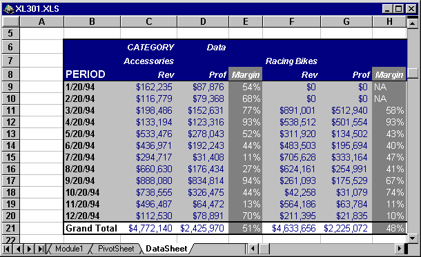
As can be seen in the diagram above, we have been able to take advantage of formulas, as well as formatting features, in the Excel worksheet to create a worksheet table that gives the impression of a pivottable—with percentage calculated fields (that even show correct values for totals).
However, with the worksheet range on the DataSheet worksheet as it currently is, we have no control over the regional data that is displayed in the worksheet table. If we add a dropdown to the worksheet, we can add a degree of control. Through use of the AddRegionDropDown2 and ChangeRegion4 macros below, we can add a dropdown to the DataSheet worksheet that allows the user to select one of four different regions. When the user selects a new region, a new SQL string is built and the pivottable is rebuilt based on the new SQL string—due to the formulas linking the DataSheet worksheet to the PivotSheet worksheet, the table on DataSheet is automatically updated when the pivottable is rebuilt.
Sub Mod1AddRegionDropDown2()
    Dim SQLString As String
    Dim PivotSheet As Worksheet
    Dim DataSheet As Worksheet
    Dim Drop1 As DropDown
    Dim Drop2 As DropDown
    Dim x As Integer
    Set DataSheet = Worksheets("DataSheet")
    Set PivotSheet = Worksheets("PivotSheet")
    Set Drop1 = PivotSheet.DropDowns("Drop1")
    SQLString = "Select Distinct Region " & _
                "From Revenue Order by Region"
    DataSheet.DropDowns.Add(49, 20, 90, 10).Name = "Drop2"
    Set Drop2 = DataSheet.DropDowns("Drop2")
    DataSheet.Select
    With Drop2
        .List = SQLRequest("DSN=SaleData", SQLString)
        .OnAction = "Mod1ChangeRegion4"
        .Placement = xlFreeFloating
        .Value = Drop1.Value
    End With
End Sub
Sub Mod1ChangeRegion4()
    Dim PivotSheet As Worksheet
    Dim DataSheet As Worksheet
    Dim Drop1 As DropDown
    Dim Drop2 As DropDown
    Dim Pivot1 As PivotTable
    Dim RegionName As String
    Dim SQLString As String
    Set PivotSheet = Worksheets("PivotSheet")
    Set DataSheet = Worksheets("DataSheet")
    Set Pivot1 = PivotSheet.PivotTables("Pivot1")
    Set Drop1 = PivotSheet.DropDowns("Drop1")
    Set Drop2 = DataSheet.DropDowns("Drop2")
    RegionName = Drop2.List(Drop2.Value)
    SQLString = "Select * From Revenue Where Region " & _
                "Like '" & RegionName & "'"
    Application.ScreenUpdating = False
    PivotSheet.Select
    Pivot1.TableRange2.Select
    PivotSheet.PivotTableWizard _
            SourceType:=xlExternal, _
            SourceData:=Array("DSN=SaleData", SQLString), _
            SaveData:=False
    DataSheet.Select
    Drop1.Value = Drop2.Value
End Sub
Using ChangeRegion4 above, we are still acting under the assumption that there is a large amount of data for any region in the pivottable—and that bringing in data for all regions will result in drains on performance. If we go back to bringing all data into the pivottable, in this case, we will actually see the data table on DataSheet update much more quickly.
Sub Mod1CreatePivot10()
    Dim Pivot1 As PivotTable
    Dim SQLString As String
    Dim PivotSheet As Worksheet
    Dim Drop1 As DropDown
    Dim DataSheet As Worksheet
    Dim x As Integer
    On Error Resume Next
    Mod1DeletePivotTables
    SQLString = "Select * From Revenue"
    Set PivotSheet = Worksheets("PivotSheet")
    Set Pivot1 = PivotSheet.PivotTableWizard _
        (SourceType:=xlExternal, _
        SourceData:=Array("DSN=SaleData", SQLString), _
        TableDestination:=PivotSheet.Range("B5"), _
        TableName:="Pivot1", _
        SaveData:=False)
    With Pivot1
        .PivotFields("Period").Orientation = xlRowField
        .PivotFields("Category").Orientation = xlColumnField
        .PivotFields("Region").Orientation = xlPageField
        With .PivotFields("Revenue")
            .Orientation = xlDataField
            .NumberFormat = "$#,##0_);($#,##0)"
            .Name = "Rev"
        End With
        With .PivotFields("Profit")
            .Orientation = xlDataField
            .NumberFormat = "$#,##0_);($#,##0)"
            .Name = "Prof"
        End With
        With .PivotFields("Data")
            .Orientation = xlColumnField
            .Position = 2
        End With
        .TableRange2.AutoFormat format:=xlClassic3
    End With
    Set DataSheet = Worksheets("DataSheet")
    Set Drop1 = DataSheet.DropDowns("Drop1")
    For x = 1 To Drop1.ListCount
        If Drop1.List(x) = _
            Pivot1.PivotFields("Region").CurrentPage Then
            Drop1.Value = x
            Exit For
        End If
    Next
    PivotSheet.DropDowns("Drop1").Delete
    Mod1CopyPivot
    Mod1InitalizeRegionDropDown3
End Sub
Sub Mod1InitalizeRegionDropDown3()
    Dim SQLString As String
    Dim DataSheet As Worksheet
    Dim Drop2 As DropDown
    Dim Pivot1 As PivotTable
    Dim PivotSheet As Worksheet
    Dim x As Integer
    Set PivotSheet = Worksheets("PivotSheet")
    Set Pivot1 = PivotSheet.PivotTables("Pivot1")
    Set DataSheet = Worksheets("DataSheet")
    SQLString = "Select Distinct Region " & _
                "From Revenue Order by Region"
    Set Drop2 = DataSheet.DropDowns("Drop2")
    With Drop2
        .List = SQLRequest("DSN=SaleData", SQLString)
        .AddItem Text:="(All)"
        .OnAction = "Mod1ChangeRegion5"
        For x = 1 To .ListCount
            If .List(x) = _
                Pivot1.PivotFields("Region").CurrentPage Then
                .Value = x
                Exit For
            End If
        Next
    End With
End Sub
Sub Mod1ChangeRegion5()
    Dim PivotSheet As Worksheet
    Dim DataSheet As Worksheet
    Dim Drop2 As DropDown
    Dim Pivot1 As PivotTable
    Dim RegionName As String
    Dim TargetRange As Range
    Set PivotSheet = Worksheets("PivotSheet")
    Set DataSheet = Worksheets("DataSheet")
    Set Pivot1 = PivotSheet.PivotTables("Pivot1")
    Set Drop2 = DataSheet.DropDowns("Drop2")
    Pivot1.PivotFields("Region").CurrentPage = _
        Drop2.List(Drop2.Value)
    Set TargetRange = DataSheet.Range("Top").CurrentRegion
    TargetRange.Columns.AutoFit
End Sub
With the table on the DataSheet worksheet, it is now possible to have calculated fields displayed for the pivottable data—no matter what grouping or totals are incorporated into the table. As an example, let's add a CheckBox to DataSheet to group the data in the Period pivotfield. Macro AddCheckBox1 below adds a checkbox to the DataSheet worksheet and assigns macro GroupPeriodField to the checkbox. Macro GroupPeriodField calls the Group method on the first cell in the DataRange of the Period pivotfield in the Row area of the pivottable—it then calls CopyPivot to copy the new pivottable structure to DataSheet.
Sub Mod1AddCheckBox1()
    Dim Check1 As CheckBox
    Dim DataSheet As Worksheet
    Set DataSheet = Worksheets("DataSheet")
    Set Check1 = DataSheet.CheckBoxes.Add(180, 20, 130, 10)
    With Check1
        .Name = "Check1"
        .Interior.ColorIndex = 15
        .OnAction = "Mod1GroupPeriodField"
        .Caption = "Display Quarterly Data"
        .Placement = xlFreeFloating
        With .Border
            .LineStyle = xlContinuous
            .ColorIndex = 1
            .Weight = xlMedium
        End With
    End With
    DataSheet.Select
End Sub
Sub Mod1GroupPeriodField()
    Dim DataSheet As Worksheet
    Dim Check1 As CheckBox
    Dim Pivot1 As PivotTable
    Dim PivotSheet As Worksheet
    Set PivotSheet = Worksheets("PivotSheet")
    Set Pivot1 = PivotSheet.PivotTables("Pivot1")
    Set DataSheet = Worksheets("DataSheet")
    Set Check1 = DataSheet.CheckBoxes("Check1")
    Application.ScreenUpdating = False
    PivotSheet.Select
    If Check1.Value = xlOn Then
        Pivot1.PivotFields("Period").DataRange.Select
        Selection.Resize(1, 1).Group _
            Start:=True, End:=True, _
            Periods:=Array(False, False, _
            False, False, False, True, False)
    Else
        Pivot1.PivotFields("Period").DataRange.Select
        Selection.Resize(1, 1).Ungroup
    End If
    Mod1CopyPivot
End Sub
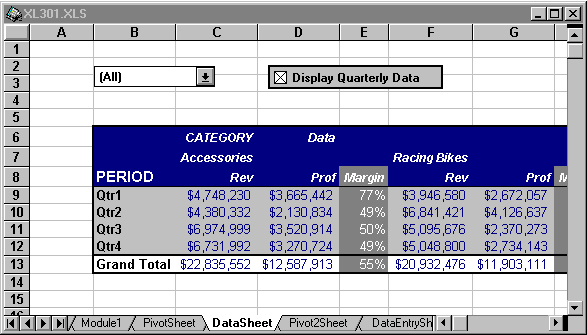
After adding the CheckBox to DataSheet—you can see how you can now group pivottable data and still have calculated fields displayed in the table on the DataSheet worksheet—as is shown in the diagram below:
You can't really enter data using a pivottable—in fact, if you try to enter data into the body of a pivottable, Excel will generate an error message indicating that data entry in a pivottable is not permitted. However, it is possible to create an interface similar to that which we created for calculated fields above that would permit this—an interface where a pivottable lies hidden in the background and data is copied from the pivottable into a worksheet that is viewed by the user. With such an interface, the user can enter data in the worksheet which can then be exported to the external data source—the pivottable cache can then be refreshed to include the data that the user has entered in the worksheet. This is a round-about way of updating the cache—however, it can prove to be an effective means of allowing a user to enter data into an external data source.
Before we go into using pivottables in such a way, let's first address one minor topic. You will have noticed that in many of the macros above, much time was spent dimensioning and setting object variables. Moving forward, instead of dimensioning and setting such object variables in every macro, let's create a single routine that can be called from any macro that will set all object variables that we will be using. In order to do this, we must declare the object variables as module-level variables. The SetObjects macro below suits our needs in this regard:
Option Explicit
Option Base 1
Dim Pivot1 As PivotTable
Dim Pivot2 As PivotTable
Dim PivotSheet As Worksheet
Dim DataSheet As Worksheet
Dim DataEntrySheet As Worksheet
Dim Pivot2Sheet As Worksheet
Dim Drop1 As DropDown
Dim ValArray() As String
Dim Check1 As CheckBox
Dim UpdateDataNow As Boolean
Dim EntryHasBeenMade As Boolean
Dim DataHasNotBeenUpdated As Boolean
Dim ValNum As Integer
Dim Button1 As Button
Dim Button2 As Button
Sub Mod2SetObjects()
    On Error Resume Next
    Set PivotSheet = Worksheets("PivotSheet")
    Set Pivot1 = PivotSheet.PivotTables("Pivot1")
    Set Pivot2Sheet = Worksheets("Pivot2Sheet")
    Set Pivot2 = Pivot2Sheet.PivotTables("Pivot2")
    Set DataSheet = Worksheets("DataSheet")
    Set DataEntrySheet = Worksheets("DataEntrySheet")
    Set Drop1 = DataEntrySheet.DropDowns("Drop1")
    Set Check1 = DataEntrySheet.CheckBoxes("Check1")
    Set Button1 = DataEntrySheet.Buttons("Button1")
    Set Button2 = DataEntrySheet.Buttons("Button2")
End Sub
Now that our object variables are set, we will need a routine that will create a second pivottable for our purposes here. Macro Mod2CreatePivot2 below creates a second pivottable on the worksheet named Pivot2Sheet—the data source for this second pivottable is the same data source as that for Pivot1 on the worksheet PivotSheet—both pivottables will actually share a common RAM cache. By sharing the data source in this manner, we can actually reduce the amount of memory stored in RAM, and improve performance:
Sub Mod2CreatePivot2()
    On Error Resume Next
    Dim SQLString As String
    Dim x As Variant
    Mod2SetObjects
    PivotSheet.Select
    Pivot1.PivotFields("Period").DataRange.Select
    Selection.Resize(1, 1).Ungroup
    Set Pivot2 = Pivot2Sheet.PivotTableWizard _
        (SourceType:=xlPivotTable, _
        SourceData:="[" & ThisWorkbook.Name & _
            "]PivotSheet!Pivot1", _
        TableDestination:=Pivot2Sheet.Range("B5"), _
        TableName:="Pivot2")
    With Pivot2
        .PivotFields("Region").Orientation = xlPageField
        .PivotFields("Period").Orientation = xlRowField
        .PivotFields("Category").Orientation = xlColumnField
        With .PivotFields("Revenue")
            .Orientation = xlDataField
            .NumberFormat = "$#,##0_);($#,##0)"
            .Name = "Rev"
        End With
        With .TableRange2
            .AutoFormat format:=xlClassic3, Width:=False
            .Columns.AutoFit
        End With
    End With
End Sub
Next, we need a macro that can be used to copy the contents of Pivot2 to a worksheet. Macro Mod2CopyPivot below copies TableRange1 of Pivot2 to worksheet DataEntrySheet. Also notice that after the copy, the macro replaces the Total values in the last row and last column with formulas—and then protects the sheet (all but the cells in the data area of the resulting table are protected). You notice that now you can enter data into the body of the resulting table on DataEntrySheet and the totals in the last row and last column will update. Attempts to enter data into any area other than the body of the table fail—sheet protection allows us to control what the user can actually change on a worksheet.
Sub Mod2CopyPivot()
    Dim RowNum As Integer
    Dim ColNum As Integer
    Dim TargetRange As Range
    Dim PivotRange As Range
    Dim x As Integer
    Dim y As Variant
    Mod2SetObjects
    Application.ScreenUpdating = False
    DataEntrySheet.Unprotect
    DataEntrySheet.Range("Top2").CurrentRegion.Clear
    With Pivot2.TableRange1
        RowNum = .Rows.Count
        ColNum = .Columns.Count
        Set TargetRange = _
        DataEntrySheet.Range("Top2").Resize(RowNum, ColNum)
    End With
    Set PivotRange = Pivot2.TableRange1
    PivotRange.Copy TargetRange
    With TargetRange
        .Columns.AutoFit
        .Offset(2, 1).Resize(RowNum - 3, ColNum - 2).Locked = _
                False
        .Offset(RowNum - 1, 1).Resize(1, 4).Formula = _
                "=sum(R[-12]C:R[-1]C)"
        .Offset(2, ColNum - 1).Resize(12, 1).Formula = _
                "=sum(RC[-3]:RC[-1])"
    End With
    With DataEntrySheet
        .Protect
        .Select
    End With
End Sub
Now, we need some way for the user to look at data for different regions. We'll add a dropdown to the DataEntrySheet worksheet that will adjust the pivottable to reflect the user's choice and then copy the resulting data to DataEntrySheet. Macro Mod2AddRegionDropDown below adds a dropdown to DataEntrySheet and then assigns the macro Mod2ChangeData to it:
Sub Mod2AddRegionDropDown()
    Dim SQLString As String
    Mod2SetObjects
    DataEntrySheet.Unprotect
    SQLString = "Select Distinct Region " & _
                "From Revenue Order by Region"
    DataEntrySheet.DropDowns.Add(49, 20, 90, 10).Name = "Drop1"
    Set Drop1 = DataEntrySheet.DropDowns("Drop1")
    DataEntrySheet.Select
    With Drop1
        .List = SQLRequest("DSN=SaleData", SQLString)
        .OnAction = "Mod2ChangeData"
        .Placement = xlFreeFloating
    End With
    DataEntrySheet.Protect
End Sub
Sub Mod2ChangeData()
    On Error Resume Next
    Dim RegionVar As String
    Dim UpdateIt As Integer
    Dim x As Variant
    Dim Drop1Val As Integer
    Mod2SetObjects
    Application.ScreenUpdating = False
    Drop1Val = Drop1.Value
    If DataHasNotBeenUpdated Then
        For x = 1 To Drop1.ListCount
            If Drop1.List(x) = _
                Pivot2.PivotFields("Region").CurrentPage Then
                Drop1.Value = x
                Exit For
            End If
        Next
        UpdateIt = MsgBox("Update changes now?", vbYesNoCancel, _
            "Update Changes?")
        If UpdateIt = vbYes Then
            Mod2UpdateDatabase
        ElseIf UpdateIt = vbCancel Then
            Exit Sub
        End If
    End If
    Drop1.Value = Drop1Val
    If EntryHasBeenMade Then
        Pivot2.RefreshTable
        EntryHasBeenMade = False
    End If
    RegionVar = Drop1.List(Drop1.Value)
    Pivot2.PivotFields("Region").CurrentPage = RegionVar
    Mod2CopyPivot
    DataHasNotBeenUpdated = False
    With Button1
        .Enabled = False
        .Font.ColorIndex = 16
    End With
End Sub
Our goal is to give the user two options:
In order to achieve this goal, we must place a checkbox on DataEntrySheet that will allow the user to choose between exporting on entry or waiting until several entries are made. We must also set an OnEntry macro that will capture the addresses of all cells into which all entries are made by the user and store such addresses in an array (valarray).
The AddCheckBox1 macro below adds a checkbox to DataEntrySheet that allows the user to select between updating external database data on entry—or waiting until a number of files have been entered, and initiating database update through clicking the Update Now button (to be added with the next macro). This is accomplished through the SetOnEntry macro assigned to the CheckBox. SetOnEntry will assign the CallUpdateDatabase macro as an OnEntry macro for the DataEntrySheet—whenever the user makes an entry on DataEntrySheet, CallUpdateDatabase will execute. Note that for the Checkbox, the Placement property is set to xlFreeFloating—because the CopyPivot macro inserts columns on DataEntrySheet, we want to make sure the checkbox is floating on the sheet to keep it from moving with the cells underneath.
Sub Mod2AddCheckBox1()
    Mod2SetObjects
    DataEntrySheet.Unprotect
    Set Check1 = DataEntrySheet.CheckBoxes.Add(180, 20, 130, 10)
    With Check1
        .Name = "Check1"
        .Interior.ColorIndex = 15
        .OnAction = "Mod2SetOnEntry"
        .Caption = "Update On Entry"
        .Placement = xlFreeFloating
        With .Border
            .LineStyle = xlContinuous
            .ColorIndex = 1
            .Weight = xlMedium
        End With
    End With
    DataEntrySheet.OnSheetActivate = "Mod2SetOnEntry"
    With DataEntrySheet
        .Protect
        .Select
    End With
End Sub
As stated above, if the Update On Entry checkbox is checked, then as the users enters data into the body of the table, entries are automatically updated to the external database (this is accomplished through the CallUpdateDatabase and UpdateDatabase macros discussed below). However, if the user does not check the Update On Entry checkbox, then addresses of cells to which the user makes changes are stored in an array called ValArray. When the user is then done making changes to data, we need a way to allow the user to update all of the changes to the external database. AddUpdateButton adds a button to DataEntrySheet that will call the UpdateDatabase macro, which will in turn update all records that correspond to the entries in ValArray.
Sub Mod2AddUpdateButton()
    Mod2SetObjects
    DataEntrySheet.Unprotect
    Set Button1 = DataEntrySheet.Buttons.Add(370, 20, 70, 25)
    With Button1
        .Name = "Button1"
        .Caption = "Update Now"
        .OnAction = "Mod2UpdateDatabase"
        .Enabled = False
        .Font.ColorIndex = 16
        .LockedText = False
    End With
    With DataEntrySheet
        .Protect
        .Select
    End With
End Sub
AddRefreshButton adds a second button to DataEntrySheet that allows the user to refresh the data in the data entry table from the external data source. This is multi-step process. Consider how the data makes its way to the table on DataEntrySheet—from the external database, data flows into the cache for Pivot1 and then into Pivot2 and is then copied to DataEntrySheet. To refresh the data then, we must call the RefreshTable method on Pivot2 (or Pivot1), then call the CopyPivot macro to copy the data from Pivot2 to DataEntrySheet.
Sub Mod2AddRefreshButton()
    Mod2SetObjects
    DataEntrySheet.Unprotect
    Set Button2 = DataEntrySheet.Buttons.Add(370, 60, 70, 25)
    With Button2
        .Name = "Button2"
        .Caption = "Refresh"
        .OnAction = "Mod2RefreshPivot"
    End With
    With DataEntrySheet
        .Protect
        .Select
    End With
End Sub
SetOnEntry below is assigned to the Update On Entry checkbox on DataEntrySheet. Depending on the value of the checkbox, SetOnEntry will assign the CallUpdateDatabase macro to the OnEntry event for DataEntrySheet and then assign a value to a module level Boolean variable named UpdateDataNow which is used to keep track of the value of the checkbox.
Sub Mod2SetOnEntry()
    On Error Resume Next
    Application.ScreenUpdating = False
    Dim x As Integer
    Mod2SetObjects
    ValNum = 1
    Select Case Check1.Value
        Case xlOn
            ReDim ValArray(1)
            UpdateDataNow = True
            DataEntrySheet.OnEntry = "Mod2CallUpdateDatabase"
        Case xlOff
            Dim TargetRange As Range
            DataEntrySheet.Unprotect
            Set TargetRange = _
                DataEntrySheet.Range("Top2").CurrentRegion
            ReDim ValArray(TargetRange.Rows.Count * _
                TargetRange.Columns.Count)
            UpdateDataNow = False
            DataEntrySheet.OnEntry = "Mod2CallUpdateDatabase"
            DataEntrySheet.Protect
    End Select
    For x = 1 To Drop1.ListCount
        If Drop1.List(x) = _
            Pivot2.PivotFields("Region").CurrentPage Then
            Drop1.Value = x
            Exit For
        End If
    Next
End Sub
CallUpdateDatabase is assigned to the OnEntry event of DataEntrySheet. Each time a user enters a value on DataEntrySheet, CallUpdateDatabase executes. CallUpdateDatabase first adds the entry just made by the user to ValArray. Then, depending on the value of the UpdateDataNow Boolean variable (the value of the Update On Entry checkbox), CallUpdateDatabase will either call the UpdateDatabase macro to update data that the user has just entered or increment the counter for ValArray—this is done so that multiple values can be added to ValArray so that all values referenced by addresses in ValArray can be updated at a later time.
Sub Mod2CallUpdateDatabase()
    On Error Resume Next
    Mod2SetObjects
    ValArray(ValNum) = ActiveCell.Address
    If UpdateDataNow Then
        Mod2UpdateDatabase
        DataHasNotBeenUpdated = False
    Else
        ValNum = ValNum + 1
        With Button1
            .Enabled = True
            .Font.ColorIndex = 1
        End With
        DataHasNotBeenUpdated = True
    End If
    EntryHasBeenMade = True
End Sub
UpdateDataBase uses all addresses in ValArray to determine into which cells in the table on DataEntrySheet entries have been made. Then by using the column heading, row heading and current selection in the dropdown on DataEntrySheet, a SQL statement is used to build a query that will update the entered value to the appropriate record in the external database. A For-Each-Next loop is used to do this for each value referenced by ValArray. Once each value has been updated, ValArray is cleared so that the whole process can start over again.
Sub Mod2UpdateDatabase()
    On Error Resume Next
    Dim Range1 As Range
    Dim TargetRange As Range
    Dim RegionVar As String
    Dim CategoryVar As String
    Dim DateVar As String
    Dim RowNum As Integer
    Dim ColNum As Integer
    Dim DataSource As Variant
    Dim SQLString As String
    Dim x As Variant
    Dim y As Integer
    Mod2SetObjects
    DataEntrySheet.Unprotect
    RegionVar = Drop1.List(Drop1.Value)
    DataSource = SQLOpen("DSN=SaleData")
    For Each x In ValArray
        If x = "" Then
            Exit For
        Else
            Set Range1 = DataEntrySheet.Range(x)
            Set TargetRange = _
                DataEntrySheet.Range("Top2").CurrentRegion
            RowNum = Range1.Row - TargetRange.Row
            ColNum = Range1.Column - TargetRange.Column
            CategoryVar = _
                TargetRange.Offset(1, ColNum).Resize(1, 1).Value
            DateVar = _
                TargetRange.Offset(RowNum, 0).Resize(1, 1).Value
            SQLString = "Update Revenue " & _
                        "Set Revenue = " & _
                        DataEntrySheet.Range(x).Value & _
                        " Where Region = '" & RegionVar & _
                        "' And Category = '" & CategoryVar & _
                        "' And Period = " & _
                        Mod2MakeDateStamp(DateVar) & ""
            SQLExecQuery DataSource, SQLString
        End If
    Next
    SQLClose DataSource
    With Button1
        .Enabled = False
        .Font.ColorIndex = 16
    End With
    DataEntrySheet.Protect
    For y = 1 To UBound(ValArray)
        ValArray(y) = ""
    Next
    ValNum = 1
    DataHasNotBeenUpdated = False
End Sub
Function MakeDataStamp is called by UpdateDatabase to convert text string dates to date stamp dates, necessary for queries involving date values with Access 2 (and SQL Server) databases.
Function Mod2MakeDateStamp(ByVal DateString As String) As String
    Dim string1 As String
    Dim YearString As String
    Dim MonthString As String
    Dim DayString As String
    Dim TempMonth As String
    Dim TempDay As String
    Dim MonthVal As Boolean
    Dim DayVal As Boolean
    Dim x As Integer
    MonthVal = True
    DayVal = False
    YearString = Right(DateString, 2)
    For x = 1 To Len(DateString)
        If DayVal = True Then
            TempDay = TempDay & Mid(DateString, x, 1)
        End If
        If Mid(DateString, x, 1) = "/" And DayVal = False Then
            MonthVal = False
            DayVal = True
        ElseIf Mid(DateString, x + 1, 1) = "/" _
            And DayVal = True Then
            DayVal = False
            Exit For
        End If
        If MonthVal = True Then
            TempMonth = TempMonth & Mid(DateString, x, 1)
        End If
    Next
    If Len(TempMonth) = 2 Then
        MonthString = TempMonth
    Else
        MonthString = "0" & TempMonth
    End If
    If Len(TempDay) = 2 Then
        DayString = TempDay
    Else
        DayString = "0" & TempDay
    End If
    string1 = "{ts '19" & YearString & "-" & _
              MonthString & "-" & _
              DayString & " 00:00:00'}"
    Mod2MakeDateStamp = string1
End Function
RefreshPivot is called by the Refresh button on DataEntrySheet. RefreshPivot first calls the RefreshTable method on Pivot2—this will update the pivottable cache that is shared between Pivot1 and Pivot2. Then, the macro copies the data from pivot2 to DataEntrySheet by using the CopyPivot macro.
Sub Mod2RefreshPivot()
    Mod2SetObjects
    Dim UpdateIt As Integer
    Application.ScreenUpdating = False
    If DataHasNotBeenUpdated Then
        UpdateIt = MsgBox("Update changes now?", vbYesNoCancel, _
            "Update Changes?")
        If UpdateIt = vbYes Then
            Mod2UpdateDatabase
        ElseIf UpdateIt = vbCancel Then
            Exit Sub
        End If
    End If
    Pivot2.RefreshTable
    Mod2CopyPivot
    With Button1
        .Enabled = False
        .Font.ColorIndex = 16
    End With
    EntryHasBeenMade = False
    DataHasNotBeenUpdated = False
End Sub
There are problems in sorting on multiple fields in the row area of a pivottable (note that no such problems exist in sorting records based on columns in the data area—this only pertains to sorting on pivotfields in the row area). Macro SecondTierSort below shows the best method to use to ensure a proper multi-tier sort. You should always sort row data in a pivottable according to the leftmost field in the row area (position 1). So to do multi-tier sorts, you must effectively, move pivotfields to position 1, perform a sort, then move the pivotfields back.
To demonstrate this, we are going to create a new pivottable. But first, we will delete the pivottable that currently exists on PivotSheet:
Sub Mod3DeletePivotTables()
    Dim x As Variant
    For Each x In Worksheets("PivotSheet").PivotTables
        x.TableRange2.Clear
    Next
End Sub
CreatePivot11 builds a new pivottable that contains two pivotfields in the row area:
Sub Mod3CreatePivot11()
    Dim Pivot1 As PivotTable
    Dim SQLString As String
    Dim PivotSheet As Worksheet
    Set PivotSheet = Worksheets("PivotSheet")
    Mod1DeletePivotTables
    SQLString = "Select * From Revenue"
    Set Pivot1 = PivotSheet.PivotTableWizard _
        (SourceType:=xlExternal, _
        SourceData:=Array("DSN=SaleData", SQLString), _
        TableDestination:=PivotSheet.Range("B5"), _
        TableName:="Pivot1", _
        SaveData:=False)
    With Pivot1
        .PivotFields("Period").Orientation = xlColumnField
        .PivotFields("Region").Orientation = xlRowField
        .PivotFields("Category").Orientation = xlRowField
        With .PivotFields("Revenue")
            .Orientation = xlDataField
            .NumberFormat = "$#,##0_);($#,##0)"
            .Name = "Rev"
        End With
        .TableRange2.AutoFormat format:=xlClassic3
    End With
End Sub
SecondTierSort sorts both pivotfields in the row area of the pivottable in a descending order. Notice how this is done however. In performing the sort, each pivotfield is moved to the first position, sorted and then moved back. In order to ensure a proper multi-tier sort of a pivottable, you must perform the sort in this manner—that is pivotfields must be sorted in the row area in position 1.
Sub Mod3SecondTierSort()
    Dim Pivot1 As PivotTable
    Dim SortRange As Range
    Set Pivot1 = Worksheets("PivotSheet").PivotTables("Pivot1")
    Worksheets("PivotSheet").Select
    Pivot1.PivotFields("Category").Position = 1
    Set SortRange = _
        Pivot1.PivotFields("Category").LabelRange.Offset(1, 0)        SortRange.Select
    SortRange.Sort order1:=xlDescending
    Pivot1.PivotFields("Region").Position = 1
    Set SortRange = _
        Pivot1.PivotFields("Region").LabelRange.Offset(1, 0)        SortRange.Select
    SortRange.Sort order1:=xlDescending
    Pivot1.PivotFields("Region").Position = 1
End Sub
The Name property of the Toolbar object in Excel is read-only—that is you cannot programmatically set the Name property. There is a way around this however. Macro ChangeToolbarName and function ChangeTBName below allow you to select a toolbar from a list of toolbars in a dropdown in a dialog box and then change that toolbars name. This is done by effectively building a second toolbar that matches the first in terms of buttons, shape and position, then deleting the original toolbar and assigning a new name to the second toolbar. Note that this routine only works for custom toolbars—you cannot change the name of a built-in toolbar.
Sub Mod4ChangeToolbarName()
    Dim Drop1 As DropDown
    Dim Edit1 As EditBox
    Dim Diag1 As DialogSheet
    Dim x As Variant
    Set Diag1 = DialogSheets("Dialog1")
    Set Drop1 = Diag1.DropDowns("Drop1")
    Set Edit1 = Diag1.EditBoxes("Edit1")
    Drop1.RemoveAllItems
    Edit1.Text = ""
    Edit1.SendToBack
    For Each x In Application.Toolbars
        Drop1.AddItem Text:=x.Name
        Drop1.Value = Drop1.ListCount
    Next
    Diag1.Show
    Mod4ChangeTBName Drop1.List(Drop1.Value), Edit1.Text
End Sub

Function Mod4ChangeTBName(ByVal Toolbar1 As String, ByVal NewName As String)
    Dim x As Variant
    Dim y As Variant
    Application.ScreenUpdating = False
    Application.Toolbars.Add NewName
    Application.Toolbars(NewName).Visible = True
    With Application
        For x = .Toolbars(Toolbar1).ToolbarButtons.Count _
                        To 1 Step -1
            .Toolbars(Toolbar1).ToolbarButtons(x).Copy _
                Toolbar:=.Toolbars(NewName), _
                before:=1
        Next
        y = .Toolbars(NewName).ToolbarButtons.Count
        For x = .Toolbars(Toolbar1).ToolbarButtons.Count _
                        To 1 Step -1
            If .Toolbars(Toolbar1).ToolbarButtons(x).IsGap Then
                .Toolbars(NewName).ToolbarButtons.Add _
                    before:=y + 1
                y = y + 1
            End If
            y = y - 1
        Next
        .Toolbars(NewName).Position = _
            .Toolbars(Toolbar1).Position
        .Toolbars(NewName).Left = .Toolbars(Toolbar1).Left
        .Toolbars(NewName).Top = .Toolbars(Toolbar1).Top
        If .Toolbars(Toolbar1).Position = xlFloating Then
            .Toolbars(NewName).Width = .Toolbars(Toolbar1).Width
        End If
        .Toolbars(Toolbar1).Delete
    End With
End Function
The UsedRange property of the worksheet object is very powerful in that it returns a rectangular range that encompasses all entered data on the worksheet. However, in Excel 5, under certain circumstances, UsedRange will return a larger range than is desired. Excel keeps track of where data exists on a worksheet. Unfortunately, if a user deletes outlying cells on a worksheet, Excel will continue to believe that such cells contain values—until the file is saved and Excel's record of the UsedRange is updated. The macros below demonstrate this problem and how to work around it. Macro SelectUsedRange1 enters data into 4 cells on worksheet ExtraSheet and then selects the sheet and then selects Used Range.
Sub Mod4SelectUsedRange1()
    With Worksheets("ExtraSheet")
        .Range("B2,C3,D4,E5").Value = 1
        .Select
        .UsedRange.Select
    End With
End Sub
The resulting range selection appears as:
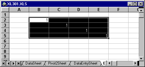
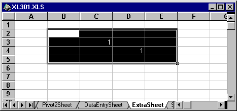
Macro SelectUsedRange2 deletes values from the two outlying cells—B2 and E5—and then selects UsedRange again:
Sub Mod4SelectUsedRange2()
    With Worksheets("ExtraSheet")
        .Range("B2,E5").Clear
        .Select
        .UsedRange.Select
    End With
End Sub
As can be seen from the diagram below, SelectUsedRange2 selects the wrong UsedRange—B2 and E5 make up the top left and bottom right corners of the range, even though they do not contain any data:
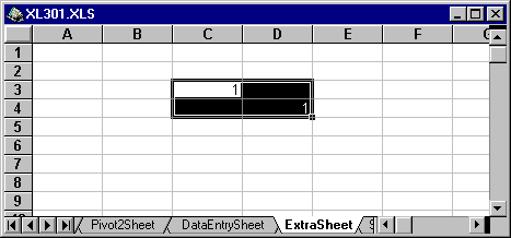
Macro SelectRealUsedRange below, combined with functions ReturnFirstCell and ReturnLastCell provide a solution to this problem. Function ReturnFirstCell obtains the top left cell in the worksheet that contains data by using UsedRange and then a series of For loops. Function ReturnLastCell uses the SpecialCells method to obtain the bottom right cell that contains data on the worksheet.
Sub Mod4SelectRealUsedRange()
    With Worksheets("ExtraSheet")
        .Select
        .Range(Mod4ReturnFirstCell(), _
            Mod4ReturnLastCell()).Select
    End With
End Sub
Function Mod4ReturnFirstCell() As String
    Dim Range1 As Range
    Dim FirstCol As Integer
    Dim FirstRow As Integer
    Dim LastCol As Integer
    Dim LastRow As Integer
    Dim x As Integer
    Dim y As Integer
    Dim r1 As Integer
    Dim r2 As Integer
    Dim r3 As Integer
    Dim c1 As Integer
    Dim c2 As Integer
    Dim c3 As Integer
    r1 = 0
    r2 = 0
    c1 = 0
    c2 = 0
    Dim FirstRowAddress As String
    Set Range1 = ActiveSheet.UsedRange
    FirstCol = Range1.Column
    FirstRow = Range1.Row
    LastCol = FirstCol + Range1.Columns.Count - 1
    LastRow = FirstRow + Range1.Rows.Count - 1
    For x = FirstRow To LastRow
        For y = FirstCol To LastCol
            If ActiveSheet.Cells(x, y).Value <> "" Then
                r1 = x
                c1 = y
                Exit For
            End If
        Next
        If r1 <> 0 Then
            Exit For
        End If
    Next
    For y = FirstCol To LastCol
        For x = FirstRow To LastRow
            If ActiveSheet.Cells(x, y).Value <> "" Then
                r2 = x
                c2 = y
                Exit For
            End If
        Next
        If r2 <> 0 Then
            Exit For
        End If
    Next
    If r1 < r2 Then
        r3 = r1
    Else
        r3 = r2
    End If
    If c1 < c2 Then
        c3 = c1
    Else
        c3 = c2
    End If
    Mod4ReturnFirstCell = ActiveSheet.Cells(r3, c3).Address
End Function
Function Mod4ReturnLastCell() As String
    Dim CurrentAddress As String
    Dim LastCellAddress As String
    CurrentAddress = ActiveCell.Address
    If Range("A1").SpecialCells(xlLastCell).Value = "" Then
        Cells(Cells.Find("*", _
            ActiveCell.SpecialCells(xlLastCell), _
            , , xlByRows, xlPrevious).Row, _
            Cells.Find("*", ActiveCell. _
            SpecialCells(xlLastCell), , , _
            xlByColumns, xlPrevious). _
            Column).Select
    Else
        Range("A1").SpecialCells(xlLastCell).Select
    End If
    LastCellAddress = Selection.Address
    Range(CurrentAddress).Select
    Mod4ReturnLastCell = LastCellAddress
End Function
As can be seen in the resulting diagram below, SelectRealUsedRange does indeed select the real used range on the worksheet:
Names are actually a rather complicated concept in Excel. I have provided several macros below to help explain some of the things that you can do with names.
First, to assign a name to a Range object, you assign a string to the Name property of the desired Range object. SetRange1 assigns the name "Range1" to Range("A1:B10") on the worksheet Sheet1—the macro then selects the sheet and uses the name to select the range:
Sub Mod5SetRange1()
    Worksheets("Sheet1").Range("A1:B10").Name = "Range1"
    Worksheets(1).Select
    Range("Range1").Select
End Sub
Note that a single Range object can have multiple names associated with it. SetRange2 below assigns the name "Range2" to the exact same range as used in the macro above. You can use the name Range2 or the name Range1 in referring to Range("A1:B10") on the worksheet Sheet1:
Sub Mod5SetRange2()
    Worksheets("Sheet1").Range("A1:B10").Name = "Range2"
    Worksheets("Sheet1").Select
    Range("Range1").Select
End Sub
To delete a name, you call the delete method on the Name object—you can reference a specific Name object by using the Names collection of the Workbook object. To index the Names collection, merely specify the name of the desired object using a string. DeleteRange1 below provides an example of deleting a name:
Sub Mod5DeleteRange1()
    ActiveWorkbook.Names("Range1").Delete
    Worksheets("Sheet1").Select
    Range("Range1").Select
End Sub
It is possible to assign a name to an offset of a range—this is accomplished by using the Offset method. The Offset method takes two arguments, a row offset and a column offset. The SetRange3 macro below assigns the name "Range3" to the cell that is 5 rows down and 5 columns to the right of Range ("A1"):
Sub Mod5SetRange3()
    Worksheets("Sheet1").Range("A1").Offset(5, 5).Name = "Range3"
    Worksheets("Sheet1").Select
    Range("Range3").Select
End Sub
In working with names, it is important that you understand the distinction between worksheet-level names and workbook-level names. Macro SetRange4 below attempts to assign the name "Range4" to two different ranges—Range("A1") on Sheet1 and Range("A1") on Sheet2. What you find happens is that once the assignment of the Range4 name on Sheet2 is made, the Range4 name on Sheet1 is deleted automatically—in this case, the name "Range4" can apply to only one range within the workbook. In this case, Range4 is a workbook-level name, in that only one instance of the "Range4" name can exist in the workbook. A call to MsgBox is made to display the address of the Range4 name by using the RefersTo property:
Sub Mod5SetRange4()
    Worksheets("Sheet1").Range("A1").Name = "Range4"
    Worksheets("Sheet2").Range("A1").Name = "Range4"
    MsgBox ActiveWorkbook.Names("Range4").RefersTo
End Sub
Using worksheet-level names, it is possible to have two identical names on two different worksheets. To accomplish this however, you must specify the worksheet name as a part of the name. Macro SetRange5 below assigns the name "Sheet1!Range5" to Range("A1") on Sheet1 and then assigns the name "Sheet2!Range5" to Range("A1") on Sheet2. The macro then uses a For-Each-Next loop to display all of the names in the workbook—you sill notice that both instances of the name Range5 exist in the workbook on separate sheets. The last two commands of the macro show how you can then use the name "Range5" in the context of the worksheet to select specific ranges:
Sub Mod5SetRange5()
    Worksheets("Sheet1").Range("A1").Name = "Sheet1!Range5"
    Worksheets("Sheet2").Range("A1").Name = "Sheet2!Range5"
    For Each x In ActiveWorkbook.Names
        MsgBox x.Name
    Next
    Worksheets("Sheet1").Select
    Range("Range5").Select
End Sub
Care should be taken not to use too many names in a workbook. You will find that using an excessive number of names (over 100) may have a negative impact on performance. This occurs because Excel registers all names in a workbook when the workbook is loaded into memory.
© 1995 Microsoft Corporation.
THESE MATERIALS ARE PROVIDED "AS-IS," FOR INFORMATIONAL PURPOSES ONLY.
NEITHER MICROSOFT NOR ITS SUPPLIERS MAKES ANY WARRANTY, EXPRESS OR IMPLIED WITH RESPECT TO THE CONTENT OF THESE MATERIALS OR THE ACCURACY OF ANY INFORMATION CONTAINED HEREIN, INCLUDING, WITHOUT LIMITATION, THE IMPLIED WARRANTIES OF MERCHANTABILITY OR FITNESS FOR A PARTICULAR PURPOSE. BECAUSE SOME STATES/JURISDICTIONS DO NOT ALLOW EXCLUSIONS OF IMPLIED WARRANTIES, THE ABOVE LIMITATION MAY NOT APPLY TO YOU.
NEITHER MICROSOFT NOR ITS SUPPLIERS SHALL HAVE ANY LIABILITY FOR ANY DAMAGES WHATSOEVER INCLUDING CONSEQUENTIAL INCIDENTAL, DIRECT, INDIRECT, SPECIAL, AND LOSS PROFITS. BECAUSE SOME STATES/JURISDICTIONS DO NOT ALLOW THE EXCLUSION OF CONSEQUENTIAL OR INCIDENTAL DAMAGES THE ABOVE LIMITATION MAY NOT APPLY TO YOU. IN ANY EVENT, MICROSOFT'S AND ITS SUPPLIERS' ENTIRE LIABILITY IN ANY MANNER ARISING OUT OF THESE MATERIALS, WHETHER BY TORT, CONTRACT, OR OTHERWISE SHALL NOT EXCEED THE SUGGESTED RETAIL PRICE OF THESE MATERIALS.