Presented by Tim Lebel
Tim Lebel is the Group Product Planning Manager with the Microsoft® Excel group helping define the future of Excel. Tim came to Microsoft in October of 1991. Prior to joining Microsoft, he spent eight years at Ashton-Tate where he worked as product manager of dBASE. In his four years at Microsoft, Tim has contributed to the launch of Microsoft Excel 4.0, 5.0, and Microsoft Excel 95 and has been a key contributor to the data access features you see today in Microsoft Excel.
Spreadsheets have grown from simple number-crunching tools into a more general purpose desktop tool for viewing as well as analyzing data. And Microsoft Excel is one of the big reasons for this. With sophisticated tools added to the spreadsheet over the years, users are now able to get at most data in an organization and utilize the spreadsheet as a tool to view and analyze that data. Microsoft Excel 5.0 contains some of the most sophisticated and powerful analysis tools available today on Personal Computers. While at Microsoft, I came across a paper written by Joel Spolsky (former design engineer for Excel) which summed it up well. It is called "A New Vision for Client/server Computing. Here is a slightly modified version of that. It can be summed up like this:
Think of all the printed reports in your company. Now think, wouldn't it be much more useful if those reports came out as Excel spreadsheets? Sure, you can print them out if you want, but you can do so much more! This is how you're going to be competitive in the next decade, and Microsoft can take you there.
The state of client/server computing today is a fraud. Client/server computing hasn't brought about the major increase in competitiveness that was promised. Today's typical client/server applications are functionally identical to their mainframe predecessors, with the addition of some pretty screen fonts.
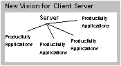
Microsoft Excel will lead a major revolution in client-server computing. We will introduce the world to a major shift in paradigm that combines the best of distributed systems with the best of personal productivity applications. This white paper introduces the philosophy that will bring about this revolution. It is a remarkable opportunity for Microsoft, if we can get it right. It means much more than Information At Your Fingertips. It is a revolutionary way that allows knowledge workers to go far beyond the traditional boundaries of how they look at data.
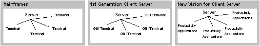
Today, when most people think of "client-server," they think of pretty GUI front-ends talking to server databases. However spiffy those front ends may be, the underlying metaphor still remains the same as it was in the days of 3270 terminals running CICS screens. This metaphor is as outdated as the computers it runs on. We need a new computing metaphor: one in which personal productivity applications, especially spreadsheets, serve as the clients in client-server systems.
In the beginning, there was ibm. And ibm made huge computers that filled up large air-conditioned rooms and required special plumbing to keep them from going up in flames. A priestly class cared for these systems in white coats. If you weren't a priest, you couldn't use the computer.
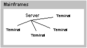
One day, someone noticed that these big computers might do a good job of keeping track of airline reservations. Imagine if reservations agents could make reservations by typing them directly into the computer! They could also check seat availability, order special meals, and even automatically send your luggage on its merry way to Kalamazoo when you're on your way to Acapulco. American Airlines had hundreds of reservations agents in those days, so they attached hundreds of terminals to their mainframes. Mainframes were the dinosaurs that ruled the earth.
The microprocessor changed all that. Personal microcomputers evolved in a radically different way than mainframes. In the PC model, Personal Productivity was the keyword. Networks and connectivity were an afterthought. Word processors, spreadsheets, and single-user databases ruled the desktop. But there was a big problem with PCs. There were still some crucial computer applications that couldn't be accomplished with PCs, such as multiuser databases and email. ibm smugly convinced itself that there would always be a market for mainframes.
This problem was solved in the 1990s, when PCs starting getting networked. All the pundits started talking about client/server computing. Client/server computing meant the end of the mainframe, because now all kinds of applications, especially multiuser databases and email, could be accomplished on networks of PCs. Yay!
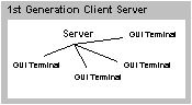
"OK," you ask. "How does this client/server stuff work?" I'll give you the classic example. Listen closely, because this is where it gets interesting. You have a multiuser application to build maybe it's email, but more likely it's a multiuser database. Here's how you build it so that it works on a network of cheapo PCs. First, put a server on a really big PC and put that in the middle of the room. Now, write client applications that have glitzy easy-to-use user interfaces, with online help, lots o' fonts, and 256 color bitmaps of the company logo. Connect clients to server with some twisted pair. Great. The client deals with the hard work of dealing with the actual user, while the server only has to actually manage the data and make sure nobody tries to do anything nasty to it.
What do client applications look like? Well, basically, they are forms-based packages. You have a form, people fill it out, then they push a button and poof all their data goes up to the server. There are lots of pretty dialogs that you can use to search, filter, and maybe even sort the data.
Look at a classic example of this client/server model: Microsoft Access. Here's what Access gives you:
Guess what? It's a big fraud. Step back for a second and ask yourself, honestly, what do PC databases do that those big bad mainframe programs didn't do? Not much. There are some pretty fonts. Maybe things are easier. It's easier to create an Access (or VB) form than it was to create a cics screen. And defining a report is much easier. That's nice. But you know what? The model is exactly the same. We still assume that people like to create big fat printed reports which list all their data in black and white. We still assume that showing one record at a time, on a screen, is the way people like to look data. Face it: an Access form is fundamentally the same as a cics screen, plus the addition of pretty fonts. An Access report is fundamentally the same as a report created in 1963 using RPG II, plus the addition of pretty fonts.
Most client/server applications are really just mainframe applications with lots o' fonts.
In the meantime, nobody seems to be asking the existential questions. Why the heck do you need printed reports, anyway? And why can't client/server applications take advantage of the real benefits of PCs (spreadsheets, word processors)?
Talk to all the people you know who have created PC database applications. Ask them if they have defined any reports. You know what? They probably haven't. Printed detail reports are honestly pretty useless.
Before you get argumentative, there are still a couple of things printed reports may be good for. Paper is still a better display medium than the screen. It is much easier to read text printed on a laser printer than to read text on the screen. But remember, we're not talking about reading Dante's Inferno, here we're talking about a detail report from a database. NOBODY reads detail reports from a database. If they do, they probably shouldn't be. So, if you really tried hard, you might convince me that printed reports are crucial for mailing labels. Whoopee. OK, so they're crucial for mailing labels. Other than that, throw them in the trash. Just build your Access application without any reports, roll it out to your users, and then decide if you really need printed reports. Betcha you don't.
In the mainframe days, people created big printed reports, but it wasn't because they wanted to read them. They printed them so that they could make big fat printouts which could be distributed to various information workers. These information workers either ignored the reports completely, or used them as a reference book, like a phone book. Sometimes they took them home so their kids could make confetti. On a very rare occasion, they would look something up. Nobody actually read the entire reports unless they were autistic like Dustin Hoffman in Rainman who read the entire phone book. So who cares if they are easier to read when they are laser printed. I'll just look up the data I need on the screen, thonk ye very much.
Which brings us to another really, really important idea. Read this twice because this idea is at the heart of where we should be going.
Online reports are infinitely more useful than printed reports.
Let's take an example of that, from real life. Last week I was looking for an apartment in Manhattan. The New York Times has about three pages, literally thousands of ads, for apartments in Manhattan. These classified ads are effectively a printed report. Let's look at how I used this report to help find an apartment.
I had some important constraints in looking for an apartment. I knew roughly the area I wanted: the West Side, somewhere between 70th and 100th street. I knew the size of apartment I could afford: about 27 square feet. And I knew a few things that I considered desirable ("vu", "drmn", "eik", "marble bath") and some things that were undesirable ("brkr", "walkup", "quaint").
Now, the New York Times apartment ads are printed in order of cross street. So I could ignore all the ads from the 1s until the 70s. But that's about all they are ordered by. So I had to read every single ad, effectively disqualifying ads as I went along. Since I was sure that I wanted to live on the West Side I skipped over all the ones that had an E next to the street number. Since I knew I couldn't afford more than about a thousand dollars, I ignored the ones that mentioned Donald Trump or Leona Helmsley. This little exercise took me a couple of hours.
Imagine that the New York Times apartment ads were delivered in Excel 5 format on a floppy disk. Wow! Now, I could narrow down my search in about five seconds using Autofilter or even just sorting by price. But I could do more interesting things, too:
Not only could I have done this, but I could have done it fairly quickly. But notice an amazing fact—typical client/server applications would not have allowed me to perform these analyses! Suppose the New York Times had hired Oracle to write an application to provide on-line classified ads. Oracle decided to do it using Visual Basic, ODBC, and Oracle 7. Sounds pretty normal. What does that VB app have? Well, I'll betcha it has two forms. The first form is a criteria screen where I'm supposed to fill in everything I'm looking for. There is a listbox to choose different neighborhoods. There are checkboxes for drmn and rvr vu. When I fill out this form, I click the OK button and I get to another screen which lists the apartments that meet the criteria I'm looking for. You know what? I'll betcha that custom $500,000 app doesn't allow me to do half of the neat things that I could do with Excel.
Anyway, hitting the pavement was getting fairly tiresome, so I finally called up a real estate broker. These are the folks who charge you literally thousands of dollars for "finding the perfect apartment." Actually, it's a big rip off. The broker I called was a company called Feathered Nest which was supposed to have hundreds of apartment listings. They were famous for having been one of the first brokers to computerize, so presumably, they could zero in on the right apartment quickly. Really? BALONEY. I told them what I wanted. They dutifully wrote it down on a piece of paper. "We'll get right back to you," they said. I was sure they would type this stuff into a computer, get back a listing of apartments that matched, and call me right back, so I sat near the phone all afternoon waiting for their call.
It took them two days to finally call me back and say, "sorry, we can't find anything that matches your requirements in the computer. You're going to have to relax your parameters." That's really what they said! "Relax your parameters." Now, this really pissed me off. "Relax This!" I said, in a close approximation of a Scottish soccer fan accent. First, they work on commission. Of COURSE they wanted me to pay more. But I knew for a fact that my parameters were not at all unreasonable; there were dozens of listings in the New York Times that matched.
But I was even more pissed off that it took them two days to plug things into the computer, and they didn't even get a very good answer back! A good answer would be, "Gee, we don't have anything that matches, but would you be willing to go as high as 96th street? There are a few apartments that match up there." Another good answer would have been "Gee, prices are so high these days on the West Side. Have you thought about living on the East Side? You could save a lot of money." A bad answer is "nothing matches, you lose." I asked them the following question: "OK, there's nothing for under $1000. So what are the lowest price apartments that are available?" They couldn't even answer this question. They kept saying "How high can you afford to go?" I don't think their computer even had an option to list the cheapest apartments. Honestly, I don't know if Feathered Nest is using a client/server computer or something a little bit more obsolete, but it sure as heck wasn't solving their customer's problems.
So, printed reports (the New York Times paper edition) suck, online client/server is hardly better, but detailed reports in Excel would be really, really nice.
Homework
Think of some database application you've worked with recently, and think about how Excel spreadsheets would be a better presentation medium than printed reports or typical client/server tools. What forms of analysis could you do that you couldn't do before? How would this provide tangible benefits?
I've illustrated that spreadsheets are the ideal medium for detailed databases for the case of apartment hunting, and in last night's homework, you came up with another example. There is a general principle involved here, and, at the risk of sounding academic, I'd like to bring it up:
Joel's Theorum: "Knowledge workers can contribute more to their organizations if they get their data as spreadsheets."
When knowledge workers get printed reports, they can't do any further analysis beyond what the designer of the report had in mind. If the New York Times doesn't have a section where it compares the average price of a 1 bedroom apartment on the East Side to the average price of a 1 bedroom apartment on the West Side, there is no way to automatically compute it. If the New York Times editors never thought it would be useful to show how much more (on average) you have to pay for a doorman building, there is no way to compute that either.
The same thing applies to business reports. If the report designer never thought it would be interesting to figure out how many pizza pies are damaged per manager, you can stare at that Damaged Pizza Report all day long and never realize that Bozo is wrecking about 3 times as many pizzas as all the other night managers put together. Knowledge workers who use printed reports will never be able to find connections, look for relationships, and track things in different ways. Thus, Joel's Theorum states quite forcefully that knowledge workers can contribute more if they get their data as spreadsheets. Companies who do this will be able to compete more effectively in a rapidly-changing world. And not just a little bit more effectively a lot more effectively.
Here's a Drama In Real Life™ to illustrate that. In the late 1980s, a decade of overbuilding caused real estate prices to collapse all over the United States. Banks that had made a lot of real estate loans were suddenly in very serious trouble. Every banker wanted to know the answer to a simple question: how much exposure do I have to real estate? Seems like an easy question, right?
As it turns out, it was an incredibly difficult question to answer! Why? Because until then, it had never occurred to anyone to create a report that showed how much exposure the bank had to different sectors. It's not that the information wasn't in the computers it was. But the report hadn't been created. For many banks, it took months to answer this simple question. One large bank in New England brought in a team of consultants for six months to figure out the answer.
Suppose the data had been easily accessible to Excel. Instead of printing a 7,000 page report listing every outstanding loan, the bank created a mongo spreadsheet listing every outstanding loan. Now, in minutes, a bank executive can figure out:
You can do this stuff easily, using AutoFilter, sorting, pivot tables, trendlines, and the usual Excel recalc stuff.
Now you can quickly start to do interesting things, like figure out if you have to tighten credit so as to prevent a cash crunch. This can all be done in minutes, in an interactive fashion. The bank executive can explore different possibilities; try what-if scenarios (what if the Yen drops? What if Dukakis is elected?) and so on and so forth. Clearly, an executive with these capabilities is going to be able to contribute more to the organization than an executive using printed reports and predefined EIS screens. Companies have to have this capability. Without it, they will not be able to compete against companies that do.
The good news is that Microsoft Excel can deliver this today. The power of Data Access and PivotTables in Excel make it easy to implement this vision.
3270
A typical "smart" terminal for ibm mainframes. See CICS.
CICS
(Pronounced "kicks".) An IBM software environment popular on mainframe systems. Under CICS, the programmer designs complete 80 x 24 screens with labels and input fields. The terminal (usually a 3270 or related terminal) is responsible for displaying the screen, filling the fields with initial values, and accepting the users input and edits. When the user presses a Send key, the entire screen of data is sent to the mainframe in a batch. This is supposed to be more efficient than UNIX™-type systems where the main CPU has to handle individual keystrokes itself. The idea is that under CICS the terminal device is smart enough to handle all the editing operations so that the mainframe only has to worry about the actual transaction processing.
Legacy Systems
Polite word for mainframes. These systems are often extremely complex and mission critical. Big companies with legacy systems would usually rather build a pretty GUI type environment around the legacy system rather than starting from scratch. See also screen scraping.
Screen Scraping
One way of putting a pretty face on legacy cics systems. The idea is that you have a fancy gui front end which acts like a virtual 3270 terminal to the back end. The front end knows exactly where the fields are on the cics forms and stuffs characters into those fields or reads it out. Theoretically, this sounds like a nice way to put some lipstick on a legacy system. In reality these projects never work very well and it is impossible to add any flexibility beyond what the underlying cics application already has.
Many thanks to Joel Spolsky (author), and he thanks Eric Michelman, Corey Salka, Adam Bosworth, Andrew Layman, Craig Unger, Andrew Kwatinetz, and Don Koscheka, without whose ideas and listening Joel's ideas would never have come this far. Special thanks to Andy Short who helped Joel reframe the question by being a great active listener.
As an added Bonus I am including a section on how to automate PivotTables in Excel 5.0. You should be sufficiently convinced by now that PivotTables in Excel and dynamic, online reports are infinitely more useful than printed reports. Here is an introduction (written last year by Eric Wells) to using VBA with PivotTables.
Sub Macro2()
ActiveSheet.PivotTableWizard SourceType:=xlDatabase, SourceData:= _
"Datasheet!$A$1:$K$226", TableDestination:= _
"'[Book2]Pivot Sheet'!R13C2", TableName:="Pivottable1", _
HasAutoFormat:=False
ActiveSheet.PivotTables("Pivottable1").AddFields RowFields:="COUNTRY", _
ColumnFields:="PRODUCT", PageFields:=Array("PROD_CAT", "REGION")
With ActiveSheet.PivotTables("Pivottable1").PivotFields("REVENUE")
.Orientation = xlDataField
.NumberFormat = "$#,##0_);($#,##0)"
End With
End SubSub Create_pivot_table()
ActiveSheet.PivotTableWizard SourceType:=xlDatabase, SourceData:= _
"Datasheet!$A$1:$K$226", TableDestination:= _
"'Pivot Sheet'!R13C2", TableName:="Pivottable1", _
HasAutoFormat:=False
ActiveSheet.PivotTables("Pivottable1").AddFields RowFields:="COUNTRY", _
ColumnFields:="PRODUCT", PageFields:=Array("PROD_CAT", "REGION")
With ActiveSheet.PivotTables("Pivottable1").PivotFields("REVENUE")
.Orientation = xlDataField
.NumberFormat = "$#,##0_);($#,##0)"
End With
range("b13").autoformat format:=xlclassic3, width:=false
End SubSub Create_pivot_table()
range("pivot_range").clear
ActiveSheet.PivotTableWizard SourceType:=xlDatabase, SourceData:= _
"Datasheet!$A$1:$K$226", TableDestination:= _
"'Pivot Sheet'!R13C2", TableName:="Pivottable1", _
HasAutoFormat:=False
ActiveSheet.PivotTables("Pivottable1").AddFields RowFields:="COUNTRY", _
ColumnFields:="PRODUCT", PageFields:=Array("PROD_CAT", "REGION")
With ActiveSheet.PivotTables("Pivottable1").PivotFields("REVENUE")
.Orientation = xlDataField
.NumberFormat = "$#,##0_);($#,##0)"
End With
range("b13").autoformat format:=xlclassic3, width:=false
dim piv as object
set piv = worksheets("pivot sheet").pivottables("pivottable1")
with piv
.pivotfields("region").currentpage = "Africa"
.pivotfields("prod_cat").currentpage = "Strings"
end with
range("a1").select
End Subsub go_to_pivot_sheet
application.screenupdating = false
worksheets("pivot sheet").select
create_pivot_table
with activewindow
.displayhorizontalscrollbar = true
.displayverticalscrollbar = true
end with
end subsub go_to_control_screen
application.screenupdating = false
worksheets("control screen").select
with activewindow
.displayhorizontalscrollbar = false
.displayverticalscrollbar = false
end with
end subSub change_pivot()
Application.ScreenUpdating = False
Dim piv As Object
Set piv = Worksheets("pivot sheet").PivotTables("pivottable1")
Dim data_output As Object
Set data_output = Worksheets("pivot sheet").Range("data_output")
piv.DataBodyRange.PivotField.Orientation = xlHidden
Select Case data_output.Value
Case 1
piv.PivotFields("revenue").Orientation = xlDataField
Case 2
piv.PivotFields("profit").Orientation = xlDataField
End Select
piv.DataBodyRange.PivotField.NumberFormat = "$#,##0_);($#,##0)"
End SubSub select_chart()
Application.ScreenUpdating = False
Dim col_chart As Object
Set col_chart = Worksheets("chart sheet").DrawingObjects("col_chart")
Dim sur_chart As Object
Set sur_chart = Worksheets("chart sheet").DrawingObjects("sur_chart")
Dim chart_selection As Object
Set chart_selection = Worksheets("chart sheet").Range("chart_selection")
Select Case chart_selection.Value
Case 1
col_chart.Top = 0
sur_chart.Top = 500
Case 2
col_chart.Top = 500
sur_chart.Top = 0
End Select
Range("a1").Select
End SubSub go_to_chart_sheet()
Application.ScreenUpdating = False
Worksheets("chart sheet").Select
With ActiveWindow
.DisplayHorizontalScrollBar = False
.DisplayVerticalScrollBar = False
End With
End SubSub go_back_to_pivot_sheet()
Application.ScreenUpdating = False
Worksheets("pivot sheet").Select
With ActiveWindow
.DisplayHorizontalScrollBar = True
.DisplayVerticalScrollBar = True
End With
End Sub Sub change_region()
Application.ScreenUpdating = False
Dim piv As Object
Set piv = Worksheets("pivot sheet") _
.PivotTables("pivottable1").PivotFields("region")
Dim region_output As Object
Set region_output = Worksheets("chart sheet").Range("region_output")
Select Case region_output.Value
Case 1
piv.CurrentPage = "Africa"
Case 2
piv.CurrentPage = "Asia"
Case 3
piv.CurrentPage = "Europe"
Case 4
piv.CurrentPage = "Latin America"
Case 5
piv.CurrentPage = "North America"
End Select
End SubDim ms_word As Object
Sub create_report()
Set ms_word = CreateObject("word.basic")
Dim piv As Object
Set piv = Worksheets("pivot sheet").PivotTables("pivottable1")
Dim col_chart As Object
Set col_chart = Worksheets("chart sheet").DrawingObjects("col_chart")
Dim data_table As Object
Set data_table = Worksheets("pivot sheet").Range("data_table")
With ms_word
.appmaximize
.filenewDefault
.insertpara
.insertpara
.Insert "Encore Musical Instruments"
.insertpara
.lineup 1
.startofline
.endofline 1
.Bold
.fontsize 18
.centerpara
.linedown 1
.insertpara
.insertpara
End With
For Each x In Worksheets("chart sheet").Range("region_input")
piv.PivotFields("region").CurrentPage = x
region_name = x.text
data_table.Copy
With ms_word
.insertpara
.insertpara
.insert (region_name)
.insertpara
.lineup 1
.startofline
.endofline 1
.bold
.fontsize 16
.linedown 1
.insertpara
.insertpara
.editpastespecial 0, 0, 0, "excel.sheet.5", "pict"
.insertpara
.insertpara
End With
col_chart.Copy
With ms_word
.editpastespecial 0, 0, 0, "excel.chart.5", "pict"
.insertbreak 0
End With
Next x
End SubSub auto_open()
Application.ScreenUpdating = False
Application.Caption = "Encore Musical Instruments"
ActiveWindow.Caption = ""
If Application.DisplayFormulaBar = True Then
Worksheets("variables").Range("formula_bar") = 1
Else
Worksheets("variables").Range("formula_bar") = 0
End If
If Application.DisplayStatusBar = True Then
Worksheets("variables").Range("status_bar") = 1
Else
Worksheets("variables").Range("status_bar") = 0
End If
Application.DisplayFormulaBar = False
Application.DisplayStatusBar = False
toolbar_num = 1
Dim toolbar_range As Object
Set toolbar_range = Worksheets("variables").Range("tool_bars")
For Each tool_bar In Application.Toolbars
If tool_bar.Visible = True Then
toolbar_range.Offset(toolbar_num, 0) = 1
Else
toolbar_range.Offset(toolbar_num, 0) = 0
End If
If (toolbar_num <> 14 And toolbar_num <> 15 _
And toolbar_num <> 16 _
And toolbar_num <> 17 And toolbar_num <> 18) Then
tool_bar.Visible = False
Else
toolbar_range.Offset(toolbar_num, 0) = 0
End If
toolbar_num = toolbar_num + 1
Next tool_bar
Worksheets("control screen").Range("a1").Select
Application.ScreenUpdating = True
End Sub Sub Auto_Close()
Application.DisplayAlerts = False
If Worksheets("variables").Range("formula_bar") = 1 Then
Application.DisplayFormulaBar = True
End If
If Worksheets("variables").Range("status_bar") = 1 Then
Application.DisplayStatusBar = True
End If
toolbar_num = 1
Dim toolbar_range As Object
Set toolbar_range = Worksheets("variables").Range("tool_bars")
For Each tool_bar In Application.Toolbars
If toolbar_range.Offset(toolbar_num, 0) = 1 Then
tool_bar.Visible = True
End If
toolbar_range.Offset(toolbar_num, 0) = 0
toolbar_num = toolbar_num + 1
Next tool_bar
Application.Caption = "Microsoft Excel"
End SubSub quit_application()
Application.DisplayAlerts = False
Application.Quit
End Sub© 1995 Microsoft Corporation.
THESE MATERIALS ARE PROVIDED "AS-IS," FOR INFORMATIONAL PURPOSES ONLY.
NEITHER MICROSOFT NOR ITS SUPPLIERS MAKES ANY WARRANTY, EXPRESS OR IMPLIED WITH RESPECT TO THE CONTENT OF THESE MATERIALS OR THE ACCURACY OF ANY INFORMATION CONTAINED HEREIN, INCLUDING, WITHOUT LIMITATION, THE IMPLIED WARRANTIES OF MERCHANTABILITY OR FITNESS FOR A PARTICULAR PURPOSE. BECAUSE SOME STATES/JURISDICTIONS DO NOT ALLOW EXCLUSIONS OF IMPLIED WARRANTIES, THE ABOVE LIMITATION MAY NOT APPLY TO YOU.
NEITHER MICROSOFT NOR ITS SUPPLIERS SHALL HAVE ANY LIABILITY FOR ANY DAMAGES WHATSOEVER INCLUDING CONSEQUENTIAL INCIDENTAL, DIRECT, INDIRECT, SPECIAL, AND LOSS PROFITS. BECAUSE SOME STATES/JURISDICTIONS DO NOT ALLOW THE EXCLUSION OF CONSEQUENTIAL OR INCIDENTAL DAMAGES THE ABOVE LIMITATION MAY NOT APPLY TO YOU. IN ANY EVENT, MICROSOFT'S AND ITS SUPPLIERS' ENTIRE LIABILITY IN ANY MANNER ARISING OUT OF THESE MATERIALS, WHETHER BY TORT, CONTRACT, OR OTHERWISE SHALL NOT EXCEED THE SUGGESTED RETAIL PRICE OF THESE MATERIALS.