In this chapter, we take the concepts that the first two chapters covered and use them to build an application in Microsoft Excel. Let's start by taking a glance at what the completed application will look like. If you have access to a computer as you read, start Excel and open the file named CHAP03-1.XLS on the companion disk packaged with this book.
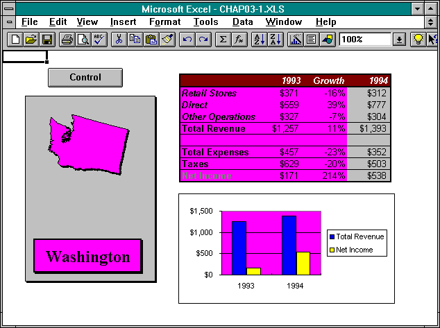
The sample application we're looking at uses as its subject a fictitious airline named West Coast Airways. West Coast Airways does business in the western United States, serving Arizona, California, Colorado, Idaho, Montana, Nevada, Oregon, Utah, Washington, and Wyoming. The application was developed solely in Excel 5 and is used by the company and specifically by its president to track summary financial data for each of the West Coast Airways sales officesthe company has one sales office in each state in which it does business. The application presents revenue and profit data in various formats for analysis, a few of which are shown in Figure 3-1 on the next page.
Users move from one format to another by choosing buttons to move to different Excel sheets, which we refer to as "forms." (The pictures and maps you see on these forms were created in drawing programs and imported as bitmaps.)

Figure 3-1. Some of the formats in which the West Coast Airways application displays data.
As soon as CHAP03-1.XLS is opened, Excel displays the main form of the application, the Control form. The Control form is used to access the various forms in the application and has several elements: a title box, some graphics, a listbox, and some buttons on a blue background.
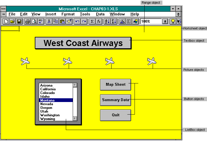
Here is a list of the objects required to create these elements:
Worksheet object: This object serves as the basis for the form; the whole area that makes up the form is, indeed, an Excel worksheet.
TextBox object: The title at the top of the screen, "West Coast Airways," is an Excel TextBox object.
Picture objects: Four Picture objects appear on the main form; these are the four small airplanes below the title.
ListBox object: The ListBox object appears in the lower left portion of the form and displays a list of the states in which the company does business. The user can select a state from the list to display sales information about that state.
Button objects: Three Button objects appear in the lower right portion of the screen: Map Sheet, Summary Data, and Quit. The user can choose these buttons either to see color-coded maps that show financial information at a glance or to quit the application.
Range object: It isn't obvious, but the Range object has been used to design this form. The blue background is a range of worksheet cells that have been colored blue so that the screen looks like a form instead of a spreadsheet.
Each state form shows summary financial information about a specific state. To display a state form, select a state from the listbox on the Control form. Selecting California from the list, for example, runs a Visual Basic for Applications (VBA) macro that activates the California form. A state form contains several Excel objects:
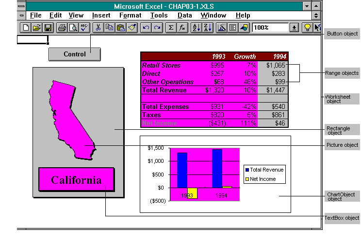
Button object: The button at the top of the sheet is the Control button; choosing it activates the Control form.
Picture object: Each state form includes a map of the selected state in the form of an imported bitmap. The maps contained in this application were created in a product called MapLand by Software Illustrated. The user can click this map to activate the map form. (See the next section.)
Rectangle object: Behind the state map is a dark gray area; this is an Excel Rectangle object that has been colored gray.
TextBox object: Beneath the map, an Excel TextBox object displays the name of the state.
Range objects: In the upper right portion of the screen, a table displays financial data specific to the selected state. This table is merely a range of cells in which data has been entered; the cells have been formatted using various colors and special effects to make them visually appealing. Note that a range of cells lies behind the other objects on the form; the gridlines have been removed to give the cells the appearance of plain white space.
ChartObject object: Below the table is a ChartObject objector what is known as an on-sheet chart. As mentioned earlier, Excel uses two types of objects for charts: a chart that floats as a graphical object on a sheetknown as a ChartObject objectand a chart that exists on a separate sheet by itselfknown as a Chart object. The ChartObject object in this case graphically displays the data from the range of cells above it and is actually linked to the cells. If the data in the cells changes, the ChartObject object is automatically updated.
Worksheet object: Again, the Worksheet object is the basis for this form.
The California form shows summary financial data for West Coast Airways business in the state of California. You'll notice that the table in the upper right displays data for the years 1993 and 1994 along with the percentage difference for various values between those two years. The chart in the lower right is linked to the table. The map of California and the textbox under the map visually key the user to the category of data being displayed on the formnamely, that for California. You'll notice that the map is color coded based on the percentage change in revenue from 1993 to 1994. If the revenue decreases by more than 20 percent, the map is red; if the change is between -20 percent and 20 percent, the map is green; if the change is greater than 20 percent, the map is blue. After reviewing the data for California, you can choose the Control button to run a macro that activates the Control form. On the Control form, try selecting some of the other states from the listbox. You'll see that each of the state forms is constructed in the same manner.
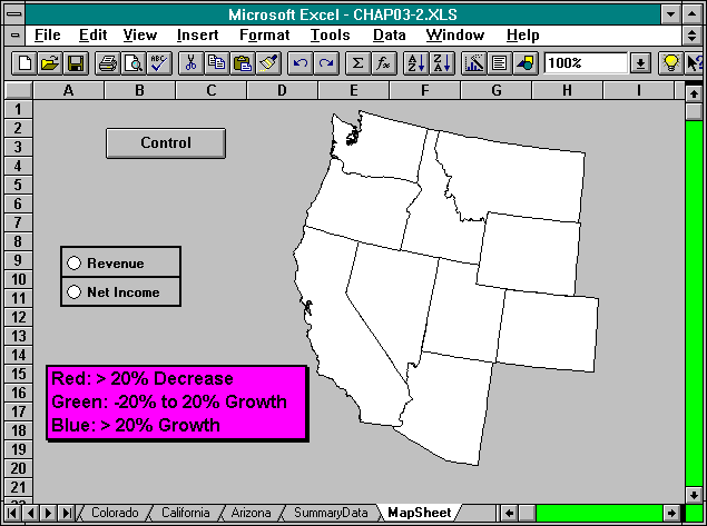
On the Control form, choose the Map Sheet button to display the map form. The map form shows a color-coded map of the western United States, which gives the user a quick view of how West Coast Airways is doing throughout the region. The map form contains these objects:
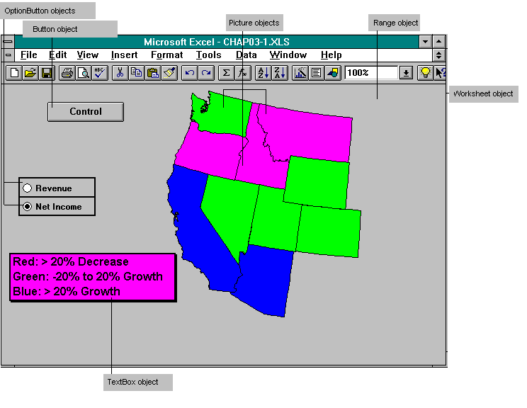
Button object: Choosing the Control button activates the Control form.
Picture objects: Ten Picture objects appear on this form; they are bitmaps, each of which depicts a state in which West Coast Airways does business. Together, they form a map of the western United States.
OptionButton objects: Two OptionButton objectsRevenue and Net Income are displayed on the left side of the form below the Control button.
TextBox object: Under the optionbuttons, a TextBox object displays a legend for the colors in the map.
Range object: A range of gray cells that lies behind the other objects.
Worksheet object: Again, the Worksheet object is the basis for this form.
The map form gives the user an immediate impression of how the company is doing in the different statesin terms of either revenue or net income (profit). By selecting either the Revenue or the Net Income optionbutton, the user launches a macro that updates the map with the appropriate data. The macro retrieves the numbers for percentage changes in revenue (growth) or net income from the state forms and colors the individual states appropriately. Try selecting the Revenue and Net Income optionbuttons now, and notice how the states change color. The user can choose the Control button to activate the Control form or click any of the individual states on the map to run a macro that activates the state form for the selected state. Try clicking some of the states on the map form now to activate the respective state forms. Recall that you can return to the map form from a state form by clicking the state map. After viewing data in the map and state forms, choose the Control button to return to the Control form.
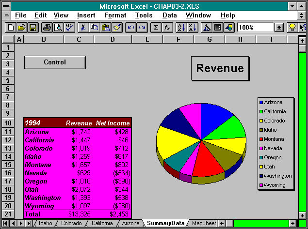
The second button on the Control form is the Summary Data button. Choose this button now to run a macro that activates the SummaryData form, which summarizes data for all of the states served by the company. The SummaryData form contains a number of objects:
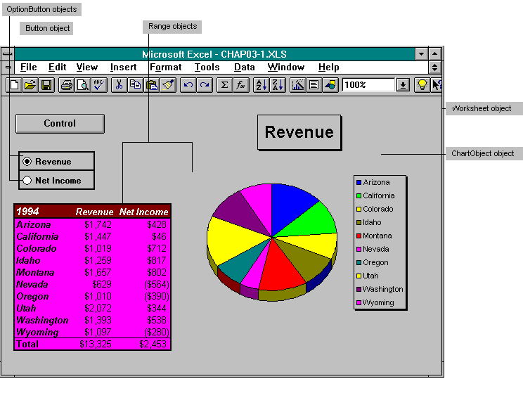
Button object: Choosing the Control button activates the Control form.
OptionButton objects: The Revenue and Net Income OptionButton objects control which type of data is displayed in the chart.
Range objects: A Range object holds the cells in the table that summarizes the data for the whole company. The table contains formulas that are linked to the individual state forms; if the data on one of the state forms changes, Excel automatically updates the table on the SummaryData form. A range of gray cells also lies behind the other objects.
ChartObject object: The on-sheet chart displays the data from the table in the form of a three-dimensional pie chart. The chart also includes a legend and a title and is automatically updated if the table changes.
Worksheet object: The Worksheet object is the basis for the form.
Selecting the Revenue or Net Income optionbutton changes the data displayed in the chart. The ChartObject object linked to the data in the table displays either "Revenue" or "Net Income" in the title above the chart. Notice the number formatting applied to the data in the table: All numbers are formatted as currency, and negative numbers are enclosed in parentheses.
Because the West Coast Airways application is such a simple one, it would probably serve best as a prototype rather than as an actual information system. Taking a critical eye to the application shows that it suffers from several flaws that would limit its use in a real-world setting.
First, the application offers no mechanism for getting data into the application other than entering it manually. Instead, the application could be set up so that the manager for each state's operation could enter data in the separate state forms and then forward the forms to the company's Finance Department viae-mail; there, the forms could be combined with the rest of the data for the West Coast Airways system. Or the state forms could use database queries that would import data from a corporate database directly into the state forms.
The second flaw involves protection of data. Nothing has been done to protect the data in the forms or the individual objects that reside on the forms. In any of the tables on the various state forms or on the SummaryData form, any user can enter any data in any of the cells. A real-world application, on the other hand, would use different levels of protection. Some elements of the application would be fully protected, and other elements would allow for different levels of access so that only certain users could change or enter certain values.
The application's third flaw lies in some of the Excel interface artifacts that are displayed on the screen. For example, unless you've changed your menu and toolbar settings manually, the standard Excel menubar with all the standard menus is displayed at the top of the Excel screen, and some Excel toolbars are visible. A professional application would not allow these or any other Excel artifacts to be displayed, in order to give the impression that a true stand-alone applicationnot an Excel macrois being used.
The fourth flaw in the application is that it does not provide any mechanism for printing or distributing data. The user could choose the Print command from the Excel File menu and print any screen; however, this possibility might not be obvious to a user who is not familiar with Excel. A professional application would provide a simple interface to allow the user to print data and might also allow the user to distribute the data over e-mail.
All of these flaws are easily eliminated by taking advantage of Excel's more advanced objectsobjects that deal with database access, control of user input, interaction with e-mail systems, and the Excel environment. We will not fix these flaws here, but in upcoming chapters in this book you will learn about the more advanced Excel objects that allow you to build a fully functional information system.
Before you close the West Coast Airways application, you should be aware of one feature we have not yet explored. If you click any of the airplane bitmaps or the title box on the Control form, you can make the airplanes "fly." For a few seconds, the four airplanes move in succession across the screen and wrap around again, giving the impression of flight. You've actually launched a macro that uses a For-Next loop to give this animated effect. After you finish watching the airplanes fly across the screen, you can choose the Quit button to close the West Coast Airways application. Quit runs a macro that closes the file that contains the application but does not exit Excel.
Shortly, we'll look at all of the macro code behind this application and even look at code that was used to build some of the application's interface elements. But first let's investigate some of the objects that this application includes.
In Chapter 1, we looked briefly at the purpose and function of a few Excel objects: Application, Workbook, Worksheet, and Range. The West Coast Airways application uses all of these objects plus a few others, most of which are graphical: Picture, ListBox, Button, Rectangle, TextBox, ChartObject, and OptionButton. All of these additional objects fall into a special class in Excel 5 known as "DrawingObject objects." In fact, a special collection called the "DrawingObjects collection" contains all of these objects, as well as some others. The DrawingObjects collection is a special collection in Excel 5 that contains objects of different types. It is itself contained in three different kinds of objects in Excel 5: Worksheet, DialogSheet, and Chart.
Note "Object A contains Object B" or "Collection A contains Object B" means that Object B is one level directly below A in the Excel object hierarchy, described in Chapter 1. Refer to Figure 1-2 on page 18, but note that the step in levels between a collection and a subobjectis illustrated quite differently from the step in levels between a singular object and a subobject. (Recall that a collection is itself a singular object and that you call a method on a collection with an index or a name argument to get to the subobjects it contains. You use a property, on the other hand, to get to a singular subobject.)
All floating graphical objects in Excel fall below the DrawingObjects collection in the Excel object hierarchy. It makes sense, then, that this collection is contained in the Worksheet, DialogSheet, and Chart objects because these three objects can serve as forms for designing user interfaces. You use objects from the DrawingObjects collection to add graphical elements and controls to such forms.
The DrawingObjects collection contains several objects, all of which are also contained in their own separate object-specific collections. Following is a list of all objects that fall beneath DrawingObjects in the Excel object hierarchy.
This list has been broken down into two different sections: "Graphical objects" and "Controls." A graphical object is used to design custom forms. A control, on the other hand, is an object that a user usually manipulates with a mouse to launch a macro.
ChartObject: An on-sheet chart that is linked to a range of data.
GroupObject: A set of objects that have been grouped together to create a single object so that all the objects can be manipulated as a unit.
OLEObject: A linked or embedded OLE object.
Drawing: A polygon created with the Excel Freeform drawing tool on the Drawing toolbar.
Picture: An imported bitmap generated in a third-party drawing program.
TextBox: A box that contains text. (A textbox can be blank.)
Label: A static text label. Labels are often used with controls.
Arc: An arc.
Line: A line.
Oval: An oval.
Rectangle: A rectangle.
Button: A button control.
CheckBox: A checkbox control that turns on and off with alternating clicks of the mouse.
DropDown: A dropdown list.
GroupBox: A box used to group OptionButton objects so that only one option can be set at a time.
ListBox: A standard listbox control.
OptionButton: An optionbutton control for which only one button in a group can be selected at a time.
ScrollBar: A scrollbar control used to increment or decrement a value by using a slider.
Spinner: A spinner control used to increment or decrement a value by clicking the up or down arrow.
EditBox: An editbox control used to enter text (on dialogsheets only).
Note All of these objects are "objects in collections" and can be accessed either from their own collections or from the DrawingObjects collection. This is similar to the Sheets and Worksheets collections; each worksheet is contained both in the Worksheets collection andalong with other types of sheetsin the Sheets collection. Being able to use either the DrawingObjects collection or a specific collection allows you to perform the same action easily on all drawingobjects or on only certain kinds of drawingobjects.
Although each of the objects in the "graphical objects" category on the preceding two pages has its own unique set of properties and methods, these objects also have a set of shared properties and methods. Below is a list of the properties that the graphical objects share. A list of the methods that the graphical objects share follows.
Border: Returns the border of the object (can be used to set the border's line style; does not apply to the Label object).
BottomRightCell: Applies only to objects on worksheets; returns the cell under the bottom right corner of the object.
Enabled: If True, the user can click the object to launch a macro if one has been assigned. If False, the user cannot launch a macro by clicking the object.
Height: The height of the object in points. (A point is 1/72 of an inch.)
Interior: Returns the interior of the object and is usually used to set the color (does not apply to the Line object).
Left: The distance in points (1/72 inch) that the object lies from the left border of the chart, worksheet, or dialogsheet on which the object resides.
Locked: If True, the user cannot manipulate the object in any way when the sheet is protected. If False, even if the sheet is protected, the object can be manipulated.
Name: The name of the object.
OnAction: The name of a macro that runs when the user clicks the object.
Placement: Can be one of three values: xlMoveAndSize (the object moves and resizes with the cells underneath it), xlMove (the object moves but does not resize with the cells underneath it), or xlFreeFloating (the object neither moves nor resizes with the cells underneath it). This property applies only to graphical objects on worksheets.
PrintObject: If True, the object is printed when a user prints the sheet. If False, the object does not appear on printouts.
RoundedCorners: If True, the object is displayed with rounded corners; if False, the object is displayed with square (90-degree-angle) corners (applies to the ChartObject, GroupObject, Rectangle, and TextBox objects only).
Shadow: If True, the object is displayed with a shadow behind it (does not apply to the Arc, Line, or Label objects).
Top: The distance in points (1/72 inch) that the object lies from the top border of the chart, worksheet, or dialogsheet on which the object resides.
TopLeftCell: Applies only to objects on worksheets; returns the cell under the top left corner of the object.
Visible: If True, the object is displayed. If False, the object is hidden from view.
Width: The width of the object in points (1/72 inch).
ZOrder: A placement order in which the object falls in the screen area in which the object resides. This order is used when objects are stacked on top of one another. A ZOrder of 1, for example, means that an object is hidden by any other object that overlaps it on the screen.
The following list shows the set of methods that graphical objects share:
BringToFront: Brings an object to the top of a three-dimensional stack of objects.
Copy: Copies the object to the clipboard.
CopyPicture: Copies the object to the clipboard as a picture.
Cut: Deletes the object and places it on the clipboard.
Delete: Deletes the object.
Duplicate: Duplicates the object (copies and pastes it in one action).
Select: Selects the object.
SendToBack: Places the object behind any overlapping objects on the screen (that is, sets the ZOrder property to 1).
Note Because all of these graphical objects share a common set of properties and methods, you have only one set of properties and methods to learn. Then the one set can be used for all of the graphical objects to which the properties and methods apply. Note that a number of the control objects in the DrawingObjects collection share some of the properties and methods listed above.
Now that we've summarized the objects that are used in the West Coast Airways application, let's build it. A good place to start is with a conceptual understanding of the flow of the application. The diagram at the top of the next page shows the various paths the user can take when navigating the West Coast Airways system:
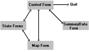
We should also consider the flow of data in the application. The data that governs the application resides in the state forms. The SummaryData form, however, contains a table in which formulas are linked to the data in the state forms, and the map form contains maps that are color coded based on the data in the state forms. Here's how data in the application flows:

We'll begin building the application by using a workbook in which some of the objects are already placed in their appropriate positions on various worksheets. Open the file CHAP03-2.XLS, which is included on the companion disk packaged with this book. After you open the file, you'll see a workbook that contains five sheets: Template, Module1, Control, SummaryData, and MapSheet. The worksheet named Template will be used as a template for making the individual state forms. Module1 will hold the VBA code for the application. Control, SummaryData, and MapSheet will be used to design the Control, SummaryData, and map forms.
Throughout the rest of this chapter, we will analyze several macros that you can use to build the application. All of these macros are contained in the text file named CHAP03.TXT. You can choose either to import the text file directly into Module1 of the file CHAP03-2.XLS and run the macros as you read or to type the macros manually as they appear in this chapter. To import the text file, click the Module1 tab to activate the module. Next choose the File command from the Insert menu, and then select CHAP03.TXT and choose OK. The code from the text file then appears in the body of the VBA module. To get the most out of this chapter, you might want to instead write the macros by yourself after reading about each macro. You can then use the code in CHAP03.TXT as a backup should you find it difficult to get your macros to run properly.
The code in this application uses arrays in a few different instances. To ensure that array indexing always starts at 1 (as opposed to 0), enter as the first line of code in Module1 an Option Base statement:
Option Base 1
You might also want to turn on forced variable declaration while writing your code. To do so, type the following statement at the top of the VBA module under the Option Base 1 statement:
Option Explicit
So far, no worksheets in the workbook represent the different state forms. We will need 10 such state form worksheets. Each worksheet will be formatted in exactly the same mannerwith a Control button, a map, a table of fictitious data, and a chart linked to that data. As a result, we can probably save time by using macros to set up the worksheets, as opposed to setting up each worksheet separately.
To help begin the process of setting up the 10 worksheets, the Template worksheet is included in the CHAP03-2.XLS workbook. Click the Template tab to take a look at it. You will notice that a formatted table in the upper right area of the worksheet depicts revenue and profit for 1993 and 1994 as well as the percentage difference for such values between the two years.
If the formula bar is not currently displayed in Excel, choose the Formula Bar command from the View menu. The formula bar is a thin bar that resides just above the worksheet (see Figure 2-1 on page 38); it serves two purposes. The right portion of the formula bar can be used to enter data and formulas in cells; the left portion of the formula bar contains the Name drop-down list box, which you can use to manually set the Name property of any range or DrawingObject object on the worksheet. (You can also use the Name box to go to a cell on the worksheet; if you select a name from the list, Excel selects the cell that matches the name.) If you look at the contents of the cells in the ranges F4:G6 and F9:G10 on the Template worksheet, you see formulas that contain the RAND() worksheet function for generating random numbers. The RAND() function has been used here merely to generate fictitious data. If you select F4:G6, the name Rand1 is displayed in the Name box; likewise, if you select F9:G10, the name Rand2 is displayed. As you will see later in this chapter, these range names will be employed in one of the macros used to set up the application. Also note that the name of cell G7 is RevenueGrowth and that the name of cell G11 is NetIncomeGrowth. (Again, cell names are displayed in the Name box.)
If you now select the MapSheet worksheet, you can see all of the states for which we need to create forms. And if you select an individual state, you can see the name of the state in the Name box. (The names of the state bitmaps, like the names of the ranges discussed in the previous section, have already been set up for you in the CHAP03-2.XLS workbook.) We can use the Name properties that are already set for the bitmaps on the MapSheet worksheet to create separate forms for each state. We would, however, like the separate state forms to appear in alphabetic order; as a result, we must sort the names of the bitmaps on the MapSheet worksheet before we use them to create the state forms. The Range object has a Sort method; if we can somehow transfer the names of the bitmaps to a worksheet range, we can sort them and then use them to create the state forms. The BuildStateList macro on the next page transfers all of the state bitmap names on the MapSheet worksheet to a range on the SummaryData worksheet and then sorts the names.
F Y I
Automated Macro Design vs. Manual Design
This chapter includes macros such as BuildStateList, below, which is used to set up your application, and macros such as GotoControl, on page 146, which is used in running your application. Often, you set up your application's environment manually, but the setup macros here serve to familiarize you with manipulating Excel objects through VBAin addition to simply helping you get your sample application running.
To distinguish between the setup macros and the macros that run your application, each setup macro in this chapter is headed "Application Setup Macro." After you run the setup macros, you no longer need to include them in Module1 in order for the application to run.
Sub BuildStateList()
    Dim TopOfList As Range
    Dim DrawVar As Drawing
    Dim Counter As Integer
    Worksheets("SummaryData").Activate
    Worksheets("SummaryData").Range("B11").Name = "TopOfList"
    Set TopOfList = Worksheets("SummaryData").Range("TopOfList")
    Counter = 11
    For Each DrawVar In Worksheets("MapSheet").Drawings
        Worksheets("SummaryData").Range("B" & Counter).Value = _
            DrawVar.Name
        Counter = Counter + 1
    Next
    TopOfList.CurrentRegion.Sort TopOfList
    TopOfList.CurrentRegion.Name = "StateList"
End Sub
In the fifth line of the BuildStateList macro, the SummaryData worksheet is made active by calling the Activate method. Then the Name property of Range("B11") on the SummaryData worksheet is set to "TopOfList", and the Set statement in the seventh line sets the TopOfList Range object to Range("TopOfList"). The For-Each-Next loop is used in the Drawings collection on the MapSheet worksheet; the Drawings collection contains all of the drawings (that is, all of the state bitmaps) on the worksheet. The statements in the For-Each-Next loop set the Value properties of cells on the SummaryData worksheet equal to the names of the drawings on the MapSheet worksheet. The list of names starts at TopOfList and then grows down one cell at a time. The Sort method is then called on the range returned by the CurrentRegion property of TopOfList. CurrentRegion is a Range property that holds a Range reference for all contiguous cells that contain data. Last, when we use the CurrentRegion property, the range that contains the sorted list is given the name StateList. Run the BuildStateList macro now to generate the sorted list.
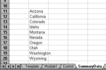
Now we'll use the sorted list on the SummaryData worksheet to make worksheets that represent a state form for each state in the list. To add the 10 worksheets that represent the forms, we'll call the Copy method on the Worksheet object to copy the Template worksheet 10 times. We'll also set the Name property of each new worksheet to the appropriate state name and then place a ChartObject object on each worksheet. The MakeSheets macro below accomplishes these tasks:
Sub MakeSheets()
    Dim StateList As Range
    Dim StateName As Range
    Set StateList = Worksheets("SummaryData").Range("StateList")
    For Each StateName In StateList
        ActiveWorkbook.Worksheets("Template").Copy ActiveSheet
        With ActiveSheet
            .Name = StateName.Value
            .Calculate
            .Range("Rand1").Copy
            .Range("Rand1").PasteSpecial xlValues
            .Range("Rand2").Copy
            .Range("Rand2").PasteSpecial xlValues
            .ChartObjects.Add(190.5, 155.25, 233.25, 118.5).Select
        End With
        ActiveChart.ChartWizard Range("E3:F3,H3," & _
                                      "E7:F7,H7," & _
                                      "E11:F11,H11")
        Range("A1").Select
    Next
End Sub
The MakeSheets macro uses a For-Each-Next loop to go through each of the cells in the StateList range, creating a new copy of the Template worksheet for each cell in the range and setting the Name property of each new worksheet to the value of each cell encountered. Notice that other things are going on in the body of the For-Each-Next loop as well. Recall that the Template worksheet contains formulas that use the RAND( ) worksheet function. By calling the Calculate method each time a new worksheet is copied, you force new random numbers to be generated, which makes it easy to create different fictitious data sets for each worksheet. After the worksheet is copied, however, you will want to convert the random formulas to actual values. You do so by calling the Range object's Copy method and then calling the PasteSpecial method, passing the constant xlValues as the first argument. This replaces all formulas in the range with the values such formulas represent (after the last recalculation). The MakeSheets macro converts the Rand1 and Rand2 ranges in this way.
Notice the call to the Add method of the ChartObjects collection. Recall that collections are actually objects that have properties and methods. In this instance, calling the Add method on the ChartObjects collection adds a new ChartObject object to the collection. Four arguments are passed to the Add method; these are values that are used to set the Left, Top, Width, and Height properties of the added ChartObject object.
In the same statement in which the Add method is called, the Select method is called as well, which ensures that the ChartObject object is selected after it has been added.
After you exit the With control structure, the ChartWizard method is called on the ActiveChart object. ActiveChart is used to reference the ChartObject object that was just added; ChartWizard is used, among other things, to link the ChartObject object to data in the worksheet. The first argument for ChartWizard takes a range address that represents the source of the linked data; in the call to ChartWizard, a series of noncontiguous ranges is specified to chart the values for Revenue and Net Income for 1993 and 1994. The last statement in the For-Each-Next loop selects the first range on the worksheet so that the ChartObject object does not remain selected.
F Y I
Using the Object Returned by the Add Method
How can you call the Add and Select methods in a single VBA statement? The Add method actually returns an objectspecifically, the new object that the method created. If you want to be able to refer to the new object again easily, you can use this fact to set a variable to the new object, as in the following:
Dim NewChart As ChartObject
Set NewChart = ActiveSheet.ChartObjects.Add(50, 20, 80, 20)
You can also use the returned object immediately, as in the following example, which sets a property and calls a method on two new objects:
ActiveSheet.ChartObjects.Add(50, 20, 80, 20).Name = "MyNewChart1"
ActiveSheet.ChartObjects.Add(80, 30, 80, 20).SendToBack
In the MakeSheets macro (see page 143) we use this feature to select the new chart and then call the ChartWizard method on the ActiveChart, but we could have also called ChartWizard directly, at the cost of making the code more cluttered and less readable.
Note that when calling the Add method, if you do not use the result in an expression (by assigning it, setting a property on it, or calling a method on it), you must either explicitly use the Call keyword or omit the parentheses from the argument list, as in the following examples:
Call ActiveSheet.ChartObjects.Add(50, 20, 80, 20)
ActiveSheet.ChartObjects.Add 50, 20, 80, 20
Tip
If you have not already done so, run the MakeSheets macro now. As each new worksheet is added and each new ChartObject object is created, you see a lot of flashing on the screen whenever something on the screen changes. You can prevent intermediate screen updatesand improve performanceby inserting the following statement at the top of the macro:
Application.ScreenUpdating = False
This statement has been omitted from the macros in this chapter so that you can see the results of property settings and method calls as they occur.
Now that you have 10 worksheets to represent the 10 state forms, you must add some of the other objects to the forms. Start by adding a Control button to each form:
Sub AddButtons()
    Dim WorksheetVar As Worksheet
    For Each WorksheetVar In ActiveWorkbook.Worksheets
        If WorksheetVar.Name <> "Control" Then
            WorksheetVar.Activate
            WorksheetVar.Buttons.Add(50, 20, 80, 20).Select
            With Selection
                .Caption = "Control"
                .OnAction = "GotoControl"
            End With
            Range("A1").Select
        End If
    Next
End Sub
The AddButtons macro above uses a For-Each-Next loop to go through each worksheet in ActiveWorkbook, adding a Button object to each worksheet except the Control worksheet. (The If statement prevents the Control worksheet from being modified.) The macro adds the Button objects by calling the Add method on the worksheet's Buttons collection. Like the ChartObjects collection, the Buttons collection has an Add method that takes four arguments; these are values that are used to set the Left, Top, Width, and Height properties of the new Button object. In the body of the For-Each-Next loop after the Button object is added, the Caption property is set to Control and the OnAction property is set to GotoControl. An object's OnAction property holds the name of a macro that is executed whenever the object is clicked. In this case, if the user chooses any of the Control buttons, the GotoControl macro is executed. Here is the macro:
Sub GotoControl()
    Worksheets("Control").Activate
    Worksheets("Control").Range("A1").Select
End Sub
This macro merely calls the Activate method on the Control Worksheet object. If you have not already done so, run the AddButtons macro now. After the macro completes, Control buttons are displayed on the 10 state forms and on the map and SummaryData forms.
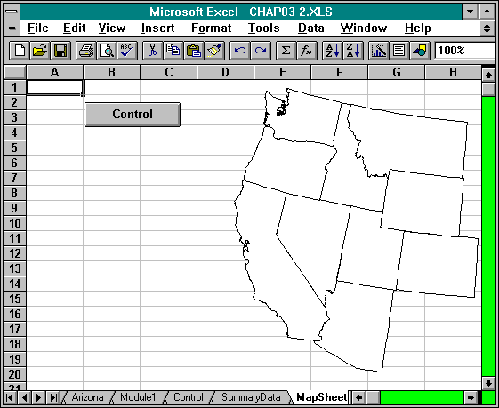
Next you need to add the map bitmaps to each of the state forms. You can do this easily by copying the bitmaps one by one from the MapSheet worksheet to the appropriate state forms. The CopyMaps macro automates the process:
Sub CopyMaps()
    Dim DrawVar As Drawing
    For Each DrawVar In Worksheets("MapSheet").Drawings
        DrawVar.Copy
        With Worksheets(DrawVar.Name)
            .Activate
            .Range("B7").Select
            .Paste
        End With
        With Selection
            If .Width <= 80 Or .Height <= 110 Then
                Do Until .Width >= 80 Or .Height >= 110
                    .Width = .Width * 1.1
                    .Height = .Height * 1.1
                Loop
            Else
                Do Until .Width < 80 Or .Height < 110
                    .Width = .Width * 0.9
                    .Height = .Height * 0.9
                Loop
            End If
            .Top = 70
            .Left = 50
            .Interior.ColorIndex = 5
            .Shadow = True
        End With
        Range("A1").Select
    Next
End Sub
Copying the state map drawings from the MapSheet worksheet to each of the state forms presents one problem: Each state map is a different size, yet on each map form you probably want the state map to appear about the same size as the other state maps. So when copying each state map, it's important to adjust the relative size of the map as it is pasted to the state form.
The first few lines in the For-Each-Next loop of the CopyMaps macro copy a state map from the MapSheet worksheet to the appropriate state form. An If-Then-Else statement then determines whether the map is too small or too large in relative terms, with the target size of each drawing set at a width of 80 points and a height of 110 points. If the state map drawing is not the correct size, one of two Do-Loops enlarges or shrinks the map until it reaches the appropriate size. The Top and Left properties of the drawing are then set to adjust the position of the state map on the form, and the ColorIndex of the Interior object is set to 5 to make each map drawing blue. The Shadow property is then set to True to give each map a shadow. Last, Range("A1") is selected so that the maps do not remain selected.
Run the CopyMaps macro. A blue drawing is displayed on each state form to depict a map of the state.
Use the following macro to add a dark gray rectangle behind each state bitmap to make it stand out:
Sub AddRectangles()
    Dim RangeVar As Range
    Dim StateList As Range
    Set StateList = Worksheets("SummaryData").Range("StateList")
    For Each RangeVar In StateList
        Worksheets(RangeVar.Value).Activate
        ActiveSheet.Rectangles.Add(25, 50, 140, 200).Select
        With Selection
            .Interior.ColorIndex = 16
            .Shadow = True
            .SendToBack
        End With
        Range("A1").Select
    Next
End Sub
In the AddRectangles macro above, a For-Each-Next loop is used on the range that the StateList object represents. The macro uses the state name in each cell in the range to activate each state form in turn. For each state form, the Add method is called on the Rectangles collection, and arguments for Left, Top, Width, and Height are passed. The ColorIndex property of the Interior object is then set to 16 to color the rectangle dark gray. Next, setting the Shadow property to True places a shadow around the rectangle. And last, the SendToBack method is called to set the ZOrder property of the rectangle to 1 so that it appears behind the graphical image of the state map.
The last object that must be added to each state form is a TextBox object, which displays the name of the state. Use the AddTextBoxes macro below to add the textboxes:
Sub AddTextBoxes()
    Dim RangeVar As Range
    Dim StateList As Range
    Set StateList = Worksheets("SummaryData").Range("StateList")
    For Each RangeVar In StateList
        Worksheets(RangeVar.Value).Activate
        ActiveSheet.TextBoxes.Add(35, 205, 115, 35).Select
        With Selection
            With .Font
                .Name = "Times New Roman"
                .Size = 18
                .Bold = True
            End With
            .Text = RangeVar.Value
            .Shadow = True
            .HorizontalAlignment = xlCenter
            .VerticalAlignment = xlCenter
            .Border.Weight = xlMedium
            .Interior.ColorIndex = 19
        End With
        Range("A1").Select
    Next
End Sub
Like the AddRectangles macro, the AddTextBoxes macro uses a For-Each-Next loop to call an Add method (this time on the TextBoxes collection) for each state form. After a textbox is added to each form, several properties of the textbox and of its font are set. The font properties that are set are Name, Size, and Bold. The following TextBox object properties are set:
|
Text |
Value of the cell in StateList |
|
Shadow |
True |
|
HorizontalAlignment |
Set to xlCenter to center the text horizontally in the box |
|
VerticalAlignment |
Set to xlCenter |
|
Border.Weight |
Set to xlMedium to give the border a medium-weight line |
|
Interior.ColorIndex |
Set to 19 to give the textbox a light yellow color |

F Y I
Automated Macro Design vs. Manual Design
The macros covered so far in this chapter have for the most part been used to create and design forms. The actions that these macros perform could have easily been accomplished manually in Excel rather than by using macros. For example, instead of using the MakeSheets macro (see page 143), you could have just as easily made 10 copies of the Template worksheet, used Excel's ChartWizard (on the Standard toolbar) to make charts on each worksheet, and then added the button, rectangle, and textbox to each worksheet by using the tools on the Drawing toolbar. Although we could perform these design tasks manually, we will continue to use macros to design the rest of the forms in this application so that you can further familiarize yourself with the objects, properties, and methods involved.
Now that all of the state forms have been designed, let's start designing the Control form by changing the background color, adding a listbox, and drawing a rectangle around the listbox. To be sure you have a feel for the pros and cons of automated vs. manual design, we list the manual steps involved in setting up this form; running the AddListBox macro on the next page, however, accomplishes the same result. In this case, only a single form is being set up, so in a real-life situation you would probably perform these steps manually, rather than spending the time to write a macro such as AddListBox.
First the background color of the Control form should be set to blue to make it appear as more of a form than a spreadsheet grid. You can do this manually by selecting the range A1:Z70, clicking the right mouse button, and then selecting Format Cells from the shortcut menu. In the Format Cells dialog box, click the Patterns tab, and then select the blue color under Cell Shading. Finish by choosing OK.
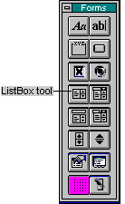
Now you need to add a listbox to the form. If the Forms toolbar is not visible, choose the Toolbars command from the View menu, check the Forms check box, and choose OK. Click the ListBox tool on the Forms toolbar and draw the listbox on the lower left portion of the screen.
To put a dark gray border around the listbox, add a rectangle behind it by first clicking the Filled Rectangle tool on the Drawing toolbar and then drawing a rectangle on top of the listbox. As with the Forms toolbar, you might need to first make the Drawing toolbar visible.

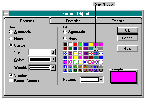
Next point to the rectangle, click the right mouse button, and select Format Object from the shortcut menu. Click the Patterns tab, and select a medium weight line from the Weight drop-down list box, check the Shadow check box, and select gray for the Fill color.
Now to place the rectangle behind the listbox, point to the rectangle, click the right mouse button, and select SendToBack from the shortcut menu.
You can also accomplish these same taskscoloring the background cells blue and adding the listbox and the rectangle behind the backgroundby running the following macro:
Sub AddListBox()
    With Worksheets("Control")
        .Select
        .Range("A1:Z70").Interior.ColorIndex = 5
        .ListBoxes.Add 100, 150, 100, 100
        .Rectangles.Add 90, 140, 120, 120
    End With
    With ActiveSheet.Rectangles(1)
        .Interior.ColorIndex = 16
        .Border.Weight = xlMedium
        .Shadow = True
        .SendToBack
    End With
End Sub
The AddListBox macro above first sets the ColorIndex property of the range's Interior object to blue, adds the listbox, adds the rectangle, and then formats the rectangle and calls the SendToBack method on the rectangle. After you add the listbox, you'll notice that no values are displayed in the list. You can choose from two ways to add a list of data so that it will be displayed in a listbox: You can link the listbox to a range on a worksheet, or you can add values to the listbox directly by using a macro. The second is the preferred wayadding values directlybecause it results in better performance than does linking the listbox to a worksheet range.
The following macro assigns the appropriate values to the listbox by storing the values directly in the listbox. To do so, the macro assigns an array to the List property; the macro also assigns another macro to the OnAction property. The OnAction macroGotoSheetis executed whenever an item is selected from the listbox.
Sub InitializeListBox()
    Dim StateList As Range
    Dim ListBox1 As ListBox
    Dim ListArray() As String
    Dim ArraySize As Integer
    Dim Counter As Integer
    Dim RangeVar As Range
    Set StateList = Worksheets("SummaryData").Range("StateList")
    Set ListBox1 = Worksheets("Control").ListBoxes(1)
    Counter = 1
    ArraySize = StateList.Rows.Count
    ReDim ListArray(ArraySize)
    Worksheets("Control").Activate
    For Each RangeVar In StateList
        ListArray(Counter) = RangeVar.Value
        Counter = Counter + 1
    Next
    With ListBox1
        .RemoveAllItems
        .List = ListArray
        .OnAction = "GotoSheet"
    End With
End Sub
The InitializeListBox macro first builds a dynamic array that contains all the values in the StateList Range object. The size of the array is determined by calling the Rows method on StateList to return the rows encompassed by StateList and then calling the Count method to get the exact number of rows. A For-Each-Next loop then goes through all the values in StateList to assign values to ListArray. Next the RemoveAllItems method is called on ListBox1 to remove any items currently in the list, and ListArray is assigned to ListBox1's List property. Last, the GotoSheet macro name is assigned to the OnAction property.
GotoSheet and ColorMap, which is called by GotoSheet, appear below:
Sub GotoSheet()
    Dim ListBox1 As ListBox
    Dim SheetName As String
    Set ListBox1 = Worksheets("Control").ListBoxes(1)
    SheetName = ListBox1.List(ListBox1.Value)
    With Worksheets(SheetName)
        ColorMap .Drawings(SheetName), "RevenueGrowth"
        .Activate
    End With
    Range("A1").Select
End Sub

Sub ColorMap(ByRef Map As Drawing, ByVal ValueName As String)
        Select Case Worksheets(Map.Name).Range(ValueName).Value
            Case Is < -0.2
                Map.Interior.ColorIndex = 3
            Case -0.2 To 0.2
                Map.Interior.ColorIndex = 4
            Case Is > 0.2
                Map.Interior.ColorIndex = 5
        End Select
End Sub
When the user selects a state from the listbox, the GotoSheet macro runs. GotoSheet retrieves the text of the item selected from the listbox in an interesting way: by indexing the list stored in the listbox. No single property of the ListBox object returns a text string that corresponds to the item selected. A ListBox object has a Value property that returns the index of the item selected and a List property that contains all of the items in the list. By using the Value property as an index on the List property, therefore, you can retrieve the text string that corresponds to the item selected. Doing so retrieves the name of the appropriate state form, which is used to call the Activate method on the worksheet that corresponds to the form.
Before the Activate method is called, a call is made to the ColorMap macro. ColorMap takes two arguments: a Drawing object passed by reference and a string passed by value. The Drawing object corresponds to the Drawing object that depicts the state map on the selected state form, and the string is "RevenueGrowth". You might recall that the cell in the state form table that contains the percentage change between 1993 and 1994 has the name RevenueGrowth. The ColorMap macro uses a Select Case statement to change the color of the map on the state form depending on the value in the cell named RevenueGrowth. If the value is less than 0.2, the map is colored red; if the value is between 0.2 and 0.2, the map is colored green; and if the value is greater than 0.2, the map is colored blue. This visual effect gives the user an immediate view of revenue growth for each state. A red map on a state form tells the user that revenue for 1994 was less than 80 percent of what it was for 1993. Likewise, a green map indicates a moderate revenue increase or decrease, and a blue map represents a high level of growth. After you run the InitializeListBox macro (see page 153), click several of the states in the listbox to see this effect.
The next major component that you need to design is the map form. To create the map form, first select the MapSheet worksheet. This worksheet includes a Control button and 10 state maps. When completed, the form will have a dark gray background, two optionbuttons for changing the map color display to either revenue or net income growth, and a textbox that displays a legend for the map colors. You can make all of these changes by running the AddMapOptionButtons and AddMapLegend macros. However, you can also design the map form manually. The process of changing the background color of the map form manually is the same as it was for the Control form: You select the cells and then select a dark gray color in the Patterns tab of the Format Cells dialog box. To add optionbuttons to the form manually, use the Option Button tool on the Forms toolbar. Last, to manually add the textbox that displays the legend, use the Text Box tool on the Drawing toolbar.
Take a look now at the AddMapOptionButtons macro, which changes the background color and adds the optionbuttons for you:
Sub AddMapOptionButtons()
    Dim CaptionArray As Variant
    Dim NameArray As Variant
    Dim ButtonCounter As Integer
    Dim TopValue As Integer
    CaptionArray = Array("Revenue", "Net Income")
    NameArray = Array("RevenueOpt", "NetIncomeOpt")
    With Worksheets("MapSheet")
        .Activate
        .Range("A1:Z70").Interior.ColorIndex = 16
        TopValue = 100
        For ButtonCounter = 1 To 2
            .OptionButtons.Add 20, TopValue, 80, 20
            With .OptionButtons(ButtonCounter)
                .Caption = CaptionArray(ButtonCounter)
                .Name = NameArray(ButtonCounter)
                .Border.Weight = xlMedium
                .Interior.ColorIndex = 15
                .OnAction = "ChangeMap"
            End With
            TopValue = TopValue + 20
        Next
    End With
End Sub
AddMapOptionButtons uses two arrays, CaptionArray and NameArray, to store the captions and names that will be assigned to the optionbuttons after they are added. After activating MapSheet, the macro sets the color of the background cells to dark gray. The macro then uses a For-Next loop to call the Add method on the OptionButtons collection twice to add two optionbuttons. Next the macro uses an index to CaptionArray and NameArray to assign values to the Caption and Name properties of the optionbuttons. Note that the Caption property refers to the text string that is displayed on the control, whereas the Name property is the name of the control as it appears in the formula bar's Name box when selected. Last the macro formats the weight of the border and the color of the interior and then assigns the ChangeMap macro name to the OnAction property. The ChangeMap macro follows:
Sub ChangeMap()
    Dim DrawVar As Drawing
    Dim DisplayValue As String
    Select Case Application.Caller
        Case "RevenueOpt"
            DisplayValue = "RevenueGrowth"
        Case "NetIncomeOpt"
            DisplayValue = "NetIncomeGrowth"
    End Select
    For Each DrawVar In Worksheets("MapSheet").Drawings
        ColorMap DrawVar, DisplayValue
    Next
End Sub
ChangeMap uses a Select Case statement with the Caller property of the Application object as the test expression. The Caller property contains the name of the object or control responsible for launching a macro. For example, the optionbuttons to which ChangeMap is assigned are named RevenueOpt and NetIncomeOpt; therefore, when ChangeMap is run, Application.Caller evaluates to either "RevenueOpt" or "NetIncomeOpt". Depending on the evaluation of the test expression, the DisplayValue string is assigned either "RevenueGrowth" or "NetIncomeGrowth". Then a For-Each-Next loop calls the ColorMap macro (described earlier, in the section titled "Working with the Control Form," beginning on page 151) to color each of the map drawings on the map form. The color assigned to each drawing depends on the level of growth of the company's revenue or net incomeas shown in the respective state forms.
F Y I
Assigning OnAction Macros Manually
After you run the AddMapOptionButtons macro, beginning on page 155, try choosing the two optionbuttons on the map form to see the colors of the maps change. Note that up to this point we have always used the OnAction property of an object to assign a macro to the object. You can also assign a macro to an object manually by pointing to the object, clicking the right mouse button, and selecting Assign Macro from the shortcut menu. After you do this, you can select a macro from the Assign Macro dialog box.
The next step is to add a legend to the map form. You can add it manually or by using the macro shown below:
Sub AddMapLegend()
    Dim LegendString As String
    LegendString = "Red: > 20% Decrease" & Chr(10) & _
                   "Green: -20% to 20% Growth" & Chr(10) & _
                   "Blue: > 20% Growth"
    With Worksheets("MapSheet")
        .Select
        .TextBoxes.Add 10, 180, 175, 50
        With .TextBoxes(1)
            .Text = LegendString
            .Interior.ColorIndex = 19
            .Border.Weight = xlMedium
            .Shadow = True
            With .Font
                .Size = 12
                .Bold = True
            End With
        End With
    End With
End Sub
Note that in the AddMapLegend macro above, two line continuation characters (a space followed by an underscore [_]) are used in the portion that assigns a text string to the LegendString variable. Also notice that the Chr function inserts a carriage return character in the string. (Macintosh users should use Chr(13) to insert a linefeed in a TextBox object.)
All of the objects have now been added to the map form.
Now you need to assign a macro to each of the state map drawings in the map form so that a user can click a state map to activate the appropriate state form. The AssignMapMacros macro below assigns the GotoStateForm macro to each state map on the map form:
Sub AssignMapMacros()
    Dim DrawVar As Drawing
    With Worksheets("MapSheet")
        .Select
        For Each DrawVar In .Drawings
            DrawVar.OnAction = "GotoStateForm"
        Next
    End With
End Sub
The GotoStateForm macro is shown at the top of the facing page. Notice how Application.Caller in GotoStateForm is used to determine the appropriate worksheet to activate after a state map is clicked. Also notice that the ColorMap macro (described earlier, in the section titled "Working with the Control Form," beginning on page 151) is called to update the color of the map on the state form so that the map displays the appropriate color for depicting revenue growth. In this application, we always call the ColorMap macro when going to a state form in case the data on which the color of the map is based ever changes.
Sub GotoStateForm()
    Dim Map As String
    Map = Application.Caller
    With Worksheets(Map)
        ColorMap .Drawings(Map), "RevenueGrowth"
        .Activate
    End With
    Range("A1").Select
End Sub
Although it is already possible to activate a state form from the map form, it should also be possible to go from a state form back to the map form. The AssignStateMapMacros macro below assigns the GotoMap macro name to the map drawings on the state forms:
Sub AssignStateMapMacros()
    Dim StateList As Range
    Dim RangeVar As Range
    Set StateList = Worksheets("SummaryData").Range("StateList")
    For Each RangeVar In StateList
        Worksheets(RangeVar.Value).Drawings(1).OnAction = "GotoMap"
    Next
End Sub
The GotoMap macro below updates all of the drawings on the map form in case any of the underlying data on the state forms has changed. To update the colors, however, it is necessary to check to see which optionbutton on the map form is currently selected; an If statement does so by checking the value of the RevenueOpt optionbutton. If the value is equal to the constant xlOn, the map colors are updated to depict revenue growth. If the value is not equal to this constant, the map colors are updated to depict net income growth.
Sub GotoMap()
    Dim DrawVar As Drawing
    Dim DisplayVal As String
    Dim RevenueOpt As OptionButton
    Set RevenueOpt = _
            Worksheets("MapSheet").OptionButtons("RevenueOpt")
    If RevenueOpt.Value = xlOn Then
        DisplayVal = "RevenueGrowth"
    Else
        DisplayVal = "NetIncomeGrowth"
    End If
    For Each DrawVar In Worksheets("MapSheet").Drawings
        ColorMap DrawVar, DisplayVal
    Next
    Worksheets("MapSheet").Select
    Range("A1").Select
End Sub
As the application looks now, a user can go from the Control form to any state form and back again and from a state form to the map form and back again. We now need to link the forms so that the user can access either the map form or the SummaryData form by choosing a button on the Control form. The Control form should also include a button for quitting the application. So we need three more buttons on the Control form.

You can add these buttons manually by using the Button tool on the Forms toolbar or by running the AddControlButtons macro:
Sub AddControlButtons()
    Dim CaptionArray As Variant
    Dim MacroArray As Variant
    Dim ButtonCounter As Integer
    Dim TopValue As Integer
    CaptionArray = Array("Map Sheet", "Summary Data", "Quit")
    MacroArray = Array("GotoMap", "GotoSummary", "QuitApp")
    With Worksheets("Control")
        .Activate
        TopValue = 140
        For ButtonCounter = 1 To 3
            .Buttons.Add 260, TopValue, 80, 30
            With .Buttons(ButtonCounter)
                .Caption = CaptionArray(ButtonCounter)
                .OnAction = MacroArray(ButtonCounter)
            End With
        TopValue = TopValue + 40
        Next
    End With
End Sub
The AddControlButtons macro uses two arraysone to hold the caption for each button and one to hold the names of the macros to assign to each button. A For-Next loop is then used to add the buttons to the form and to assign the appropriate captions and macros. The macros that are launched by the SummaryData and Quit buttons are shown below:
Sub GotoSummary()
    Worksheets("SummaryData").Select
    Range("A1").Select
End Sub

Sub QuitApp()
    ActiveWorkbook.Close
End Sub
So far, you've done little to the SummaryData form, which currently holds only a list of state names. The completed SummaryData form, however, should contain a table that lists revenue and profit figures for each state, a chart that's linked to the table, and two optionbuttons that let the user toggle between revenue and net income data in the chart. The BuildTable macro shown below builds and formats the table. (You can also build and format this table manually.)
Sub BuildTable()
    Dim TopOfList As Range
    Dim StateList As Range
    Dim StateName As Range
    Dim StCnt As Integer
    Set TopOfList = Worksheets("SummaryData").Range("TopOfList")
    Set StateList = Worksheets("SummaryData").Range("StateList")
    With Worksheets("SummaryData")
        .Activate
        .Range("A1:Z70").Interior.ColorIndex = 16
    End With

    'Add a formula in the cells--for example, =Arizona!Revenue
    StCnt = 0
    For Each StateName In StateList
        StateName.Offset(0, 1).Formula = _
                "=" & StateName.Value & "!Revenue"
        StateName.Offset(0, 2).Formula = _
                "=" & StateName.Value & "!Net_Income"
        StCnt = StCnt + 1
    Next

    'Add headings, totals formulas, and cell formatting
    With TopOfList
        'Column headings:
        .Offset(-1, 0).Value = "'1994"
        .Offset(-1, 1).Value = "Revenue"
        .Offset(-1, 2).Value = "Net Income"

        'Row heading and totals formulas on bottom row:
        .Offset(StCnt, 0).Value = "Total"
        .Offset(StCnt, 1).FormulaR1C1 = _
                "=SUM(R[-" & StCnt & "]C:R[-1]C)"
        .Offset(StCnt, 2).FormulaR1C1 = _
                "=SUM(R[-" & StCnt & "]C:R[-1]C)"

        'Cell formatting:
        .CurrentRegion.NumberFormat = "$#,##0_);($#,##0)"
        .CurrentRegion.AutoFormat Format:=xlColor2
        .CurrentRegion.BorderAround , xlMedium
    End With
    Worksheets("SummaryData").Columns(1).ColumnWidth = 2
End Sub
This macro takes advantage of several features of the Range object that have not yet been discussed; we'll look at those here. The first With statement activates the SummaryData worksheet and colors the background cells dark gray.
Next a For-Each-Next loop goes through StateList row by row, using the Range object's Offset method to refer to neighboring cells and assigning values to the Formula properties of those cells. Offset takes two arguments: a row number and a column number. The first call to Offset returns the cell that is one column to the right in the same row as the current cell in StateList. The Formula property is then set for this cell to a formula that evaluates to "=StateName!Revenue". This formula links the cell to the cell named Revenue on the appropriate state form. For example, in the California row of the table, this formula would be "=California!Revenue". Note that all Excel worksheet formulas that involve links to cells on other worksheets adhere to this syntax: a worksheet name followed by an exclamation point, and then either a cell address or a cell name. The next statement in the For-Each-Next loop performs a similar action: setting the Formula property of the cell in the next column equal to "=StateName!NetIncome". This formula links the cell to the NetIncome cell on the appropriate state form.
The block of code inside the With statement after the For-Each-Next loop adds headings and formats and fills in the bottom row with totals for the Revenue and Net Income columns. Labels are added using the Offset method and Value property of a Range object. The totals are created by setting the Formula properties of the respective cells to a SUM formula that calculates the sum of all numbers in the rows of that particular table column. The SUM formula takes a Range argument, specified here by a starting cell address and an ending cell address, with the two separated by a colon. The SUM formulas used in the BuildTable macro use relative addresses, in which row and column number offsets are specified. The exact syntax of the SUM formula is "=SUM(R[-" & StCnt & "]C:R[-1]C)", where StCnt represents the number of rows that contain data. The formula can be read as "sum the values starting at StCnt rows up in the same column and ending one row up in the same column." Note that because no column offset is specified, it is assumed to be zero.
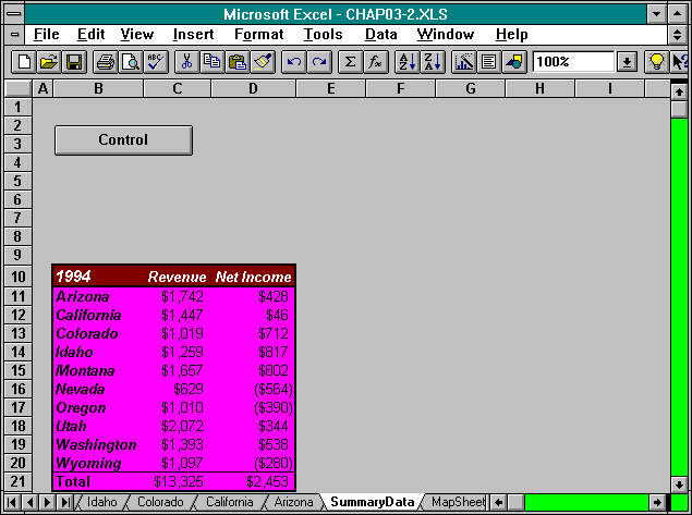
After the macro enters the SUM formulas in the bottom row of the table, it formats the entire table. The NumberFormat property of the range that encompasses the table is set to a currency format, and the AutoFormat method is called on the range to apply a built-in format named xlColor2. Last the macro places a solid border of medium weight around the table and sets the ColumnWidth property of the worksheet's first column to 2 to reduce the width of the form's left margin, as shown here:
Next you need to add a chart to the SummaryData form. You would typically create a single on-sheet chart manually by using the ChartWizard tool on the Standard toolbar. The CreateChart macro shown below adds a chart for you automatically:
Sub CreateChart()
    Dim TableRange As Range
    Dim RevenueRange As Range
    Dim NetIncomeRange As Range
    Dim R1 As Range
    Dim R2 As Range
    Dim FirstRow As Integer
    Dim FirstColumn As Integer
    Dim LastRow As Integer
    Dim LastColumn As Integer

    Worksheets("SummaryData").Activate

    'TableRange is the entire table
    Set TableRange = Worksheets("SummaryData").Range("TopOfList") _
                     .CurrentRegion

    'Make it easy to refer to the boundaries of the table
    FirstRow = TableRange.Row
    FirstColumn = TableRange.Column
    LastRow = TableRange.Rows.Count + FirstRow - 1
    LastColumn = TableRange.Columns.Count + FirstColumn - 1

    'Point to and name the revenue portion of the table
    '(including row headings but not including totals)
    Set RevenueRange = Worksheets("SummaryData").Range( _
                            Cells(FirstRow, FirstColumn), _
                            Cells(LastRow - 1, LastColumn - 1))
    RevenueRange.Name = "RevenueRange"

    'R1 is the range that holds row headings (but not "Total"),
    'R2 is the range that holds NetIncome values (but not total)
    Set R1 = Range(Cells(FirstRow, FirstColumn), _
                   Cells(LastRow - 1, LastColumn - 2))
    Set R2 = Range(Cells(FirstRow, FirstColumn + 2), _
                   Cells(LastRow - 1, LastColumn))

    'Point to and name the net income portion of the table
    '(including row headings but not including totals)
    Set NetIncomeRange = Union(R1, R2)
    NetIncomeRange.Name = "NetIncomeRange"

    'Add a chart that's linked to RevenueRange
    RevenueRange.Select
    ActiveSheet.ChartObjects.Add(198.75, 12, 240, 243).Select
    ActiveChart.ChartWizard source:=RevenueRange, _
                            gallery:=xl3DPie, _
                            format:=1, _
                            plotBy:=xlColumns, _
                            categoryLabels:=1, _
                            seriesLabels:=1

    'Format the new chart
    Worksheets("SummaryData").ChartObjects(1).Activate
    With ActiveChart
        .Elevation = 55
        .Legend.Shadow = True
        .Legend.Interior.ColorIndex = 15
        .ChartTitle.Font.Size = 18
        .ChartTitle.Font.Bold = True
        .ChartTitle.Border.LineStyle = xlMedium
        .ChartTitle.Shadow = True
        .ChartTitle.Interior.ColorIndex = 15
    End With

    'Deactivate the chart by hiding the ActiveWindow
    ActiveWindow.Visible = False
    With Worksheets("SummaryData").ChartObjects(1)
        .Border.LineStyle = xlNone
        .Interior.ColorIndex = 16
    End With
    Worksheets("SummaryData").Range("A1").Select
End Sub
The CreateChart macro above selects the appropriate data range in the table that is on the SummaryData form, calls the Add method of the ChartObjects collection to add an on-sheet chart, and then calls the ChartWizard method to link the chart to the appropriate range in the table. The CreateChart macro then activates the chart and formats various properties of the chart itself.
The first portion of the CreateChart macro is rather complicated because the first two columns of the table (excluding the last row, which contains totals) must be selected before the macro can call the Add method of the ChartObjects collection. We know that the cell at the top of the list of states is named TopOfList. The eighth line of the macro sets the TableRange variable equal to the range that corresponds to the CurrentRegion property of the TopOfList range; this is actually the entire table. (The line continuation character [_] is used in the statement to carry it over to the next line.) The next four statements set integer variables that reference the table's first and last rows and first and last columns.
The RevenueRange object variable is then set equal to the range in the table that corresponds to the table's first two columns, excluding the last row. The statement uses the Range object and the Cells method. Cells takes two argumentsa row number and a column numberand returns a single cell that represents the intersection of the row and column numbers on the worksheet. The Cells method can be called on the Application, Worksheet, or Range object. In this case, the call is made on the Application object. (Application is the default when no object is specified.) Because Cells is called on the Application object here, the appropriate worksheet must be active at the time, which is why the Activate method is called on the SummaryData Worksheet object at the beginning of the macro.
Note that when called from a worksheet, Range acts as a method that returns a Range object and can take as arguments either a single range address or two individual cell addresses. When Range takes two cell addresses as arguments, the range that is returned is the entire range that falls between those two cells. By using the Range and Cells methods in conjunction, you can set the RevenueRange object to the table's first two columns, excluding the last row. A name is then assigned to the range so that this complicated process need not be repeated the next time you want to select this range.
The next set of statements are more complicated yet. They involve selecting a range of data to be used to chart net income values. Such a chart requires selecting the first and last columns of the table, excluding the last row. The chart created in the CreateChart macro displays revenue values. However, a range for charting net income will also be set in this macro to be used by the ChangeChart macro (described in the next section). The ChangeChart macro is called by the optionbuttons that you still must add to the SummaryData form. ChangeChart allows the user to change which set of data is linked to the chart. To set NetIncomeRange, two range variables, R1 and R2, are used. Again, by using the Range and Cells methods, R1 is set to the table's first column, excluding the last row, and R2 is set to the table's last column, excluding the last row. Then the Union function combines R1 with R2 and assigns the union to the NetIncomeRange variable. The range is then given a name so that it can be accessed easily in the future.
After all this complicated manipulation of ranges, RevenueRange is selected, and the Add method is called on the ChartObjects collection to add a chart to the form. Next the macro calls the ChartWizard method on the new chart to link it to RevenueRange. Notice that several other arguments are passed to the ChartWizard method to specify values for various properties of the chart. After the chart is linked to the worksheet, the chart is activated so that additional properties of the chart can be set, including the elevation of the chart and various properties of the Legend and ChartTitle objects. The chart is then deactivated when the macro sets the Visible property of the ActiveWindow object to False. Last the line style of the border and the color of the interior of the chart are set. The line style is set to xlNone so that no border appears, and the color is set to dark gray to make the chart blend in with the background.
You now need to add the two optionbuttons that allow the user to choose between displaying revenue information and displaying net income information on the chart. The AddChartOptionButtons macro below adds the two optionbuttons to the SummaryData form and sets the OnAction property of each optionbutton to the ChangeChart macro:
Sub AddChartOptionButtons()
    Dim CaptionArray As Variant
    Dim NameArray As Variant
    Dim ButtonCounter As Integer
    Dim TopValue As Integer
    CaptionArray = Array("Revenue", "Net Income")
    NameArray = Array("RevenueChart", "NetIncomeChart")
    With Worksheets("SummaryData")
        .Select
        TopValue = 60
        For ButtonCounter = 1 To 2
            .OptionButtons.Add 20, TopValue, 80, 20
            With .OptionButtons(ButtonCounter)
                .Caption = CaptionArray(ButtonCounter)
                .Name = NameArray(ButtonCounter)
                .Border.Weight = xlMedium
                .Interior.ColorIndex = 15
                .OnAction = "ChangeChart"
            End With
            TopValue = TopValue + 20
        Next
    End With
End Sub
The AddChartOptionButtons macro is nearly identical to the AddMapOptionButtons macro discussed earlier, in the section titled "Working with the Map Form," beginning on page 155. We will not, therefore, look at AddChartOptionButtons in detail. However, the ChangeChart macro, which allows the user to change data that has been charted, appears below. It is assigned to the optionbuttons on the SummaryData form.
Sub ChangeChart()
    Dim RevenueRange As Range
    Dim NetIncomeRange As Range
    Set RevenueRange = Worksheets("SummaryData").Range("RevenueRange")
    Set NetIncomeRange = Worksheets("SummaryData").Range("NetIncomeRange")
    Worksheets("SummaryData").ChartObjects(1).Select
    Select Case Application.Caller
        Case "RevenueChart"
            ActiveChart.ChartWizard source:=RevenueRange
        Case "NetIncomeChart"
            ActiveChart.ChartWizard source:=NetIncomeRange
    End Select
    Worksheets("SummaryData").Range("A1").Select
End Sub
The ChangeChart macro above employs a Select Case statement that uses Application.Caller as the test expression. If the RevenueChart optionbutton is selected, RevenueRange is passed as the source argument to the ChartWizard method, and revenue data is displayed on the chart. If the NetIncomeChart optionbutton is selected, however, NetIncomeRange is passed as the source argument to ChartWizard, and net income data is displayed on the chart.
The application is now nearly complete. Still missing are two elements on the Control form: the title textbox and the airplane graphics.
You can use the AddAppTitleBox macro below to add the title textbox:
Sub AddAppTitleBox()
    Dim TitleString As String
    TitleString = "West Coast Airways"
    Worksheets("Control").Select
    ActiveSheet.TextBoxes.Add 90, 30, 250, 30
    With ActiveSheet.TextBoxes(1)
        .Text = TitleString
        .Interior.ColorIndex = 15
        .Border.Weight = xlMedium
        .Shadow = True
        .Font.Size = 22
        .Font.Bold = True
        .HorizontalAlignment = xlCenter
        .VerticalAlignment = xlCenter
    End With
    Range("A1").Select
End Sub
AddAppTitleBox merely calls the Add method on the TextBoxes collection and sets various properties of the added textbox.
Now you're ready to insert the Picture objects that represent the bitmaps of the airplanes flying across the screen. A file named PLANE.BMP on the companion disk packaged with this book contains a bitmap of an airplane. To insert the bitmap file in the Control form manually, choose the Picture command from the Insert menu, and then select the PLANE.BMP file.
Note
Excel's Picture command (found on the Insert menu in Windows) is not available on the Macintosh. The CHAP03-2.XLS file on the Macintosh disk (available from Microsoft Press through a fulfillment order) contains a bitmap picture of an airplane already. Macintosh users should use this bitmap rather than the PLANE.BMP file. The InsertPlanes macro on the Macintosh disk omits the code for inserting the PLANE.BMP file and uses the following line of code in place of the With Selection statement:
With ActiveSheet.Pictures(1)
See the section titled "Using the Companion Disk," beginning on page xxvii, for instructions on ordering the Macintosh fulfillment disk.
Make three additional copies of the Picture object, and space them evenly across the form immediately below the application title box. The InsertPlanes macro below automates the process of inserting the bitmap, making the copies, and spacing the objects evenly. (This macro assumes that the PLANE.BMP file is saved in the same directory as is the workbook in which the macro is being run: ThisWorkbook.)
Sub InsertPlanes()
    Dim PlaneCounter As Integer
    Dim LeftValue As Integer
    Dim PathString As String
    Dim DirectoryVar As String
    DirectoryVar = Application.PathSeparator
    PathString = ThisWorkbook.Path & DirectoryVar & "PLANE.BMP"
    Worksheets("Control").Activate
    ActiveSheet.Pictures.Insert(PathString).Select
    With Selection
        .Border.LineStyle = xlNone
        .Copy
    End With
    For PlaneCounter = 1 To 3
        ActiveSheet.Paste
    Next
    LeftValue = 50
    For PlaneCounter = 1 To 4
        With Worksheets("Control").Pictures(PlaneCounter)
            .Left = LeftValue
            .Top = 80
            .OnAction = "FlyPlanes"
            LeftValue = LeftValue + 110
        End With
    Next
    Worksheets("Control").TextBoxes(1).OnAction = "FlyPlanes"
    Range("A1").Select
End Sub
In the InsertPlanes macro, the string DirectoryVar is set to Application.PathSeparator, which returns the correct operating system path separator regardless of whether the macro is run on a Macintosh or in Windows (either ":" or "\"). You then build the path for the PLANE.BMP file by appending the directory separator and the PLANE.BMP filename to the end of the string returned by ThisWorkbook.Path. This happens to be the path to which the current workbook file is saved. You then insert the PLANE.BMP bitmap by calling the Insert method on the Pictures collection, and continue by setting the LineStyle property of the Border object to xlNone to take away the border around the picture. The picture is then copied to the clipboard. Next a For-Next loop pastes the picture three times so that you now have four pictures on the Control form. A For-Each-Next loop then spaces the four pictures evenly in a horizontal line across the form below the application title box. It does so by setting the Left and Top properties of each picture appropriately. The OnAction property of each picture is set to the FlyPlanes macro, and at the end of the macro, the OnAction property of the application's title TextBox object is also set to FlyPlanes. The FlyPlanes macro appears below:
Sub FlyPlanes()
    Dim DrawVar As Picture
    Dim FlightCounter As Integer
    Dim Counter As Integer
    For Counter = 1 To 4
        Worksheets("Control").Pictures.Group
        With Worksheets("Control").GroupObjects(1)
            For FlightCounter = 1 To 6
                .Left = .Left + 10
            Next
            .Ungroup
        End With
        For Each DrawVar In Worksheets("Control").Pictures
            If DrawVar.Left > 355 Then
                DrawVar.Left = 0
            End If
        Next
        Worksheets("Control").Pictures.Group
        With Worksheets("Control").GroupObjects(1)
            For FlightCounter = 1 To 5
                .Left = .Left + 10
            Next
            .Ungroup
        End With
    Next
    Range("A1").Select
End Sub
FlyPlanes first calls the Group method on the Control form's Pictures collection. Doing so groups all the airplane bitmap pictures together so that they can be treated as a single objectthat is, as a GroupObject object. This single object is then referenced as GroupObjects(1), and a For-Next loop moves the group 60 points horizontally across the screen in an animated fashion by incrementing the Left property of the group. The Ungroup method is then called on the group to again break it into four separate Picture objects. The macro then moves the Picture object that is on the far right back to the far left by setting the Left property to 0. The objects are grouped again and then moved 50 more points across the screen to the right. Last the Ungroup method is called on the group so that FlyPlanes will work the next time it is called.
The Control form is now complete.
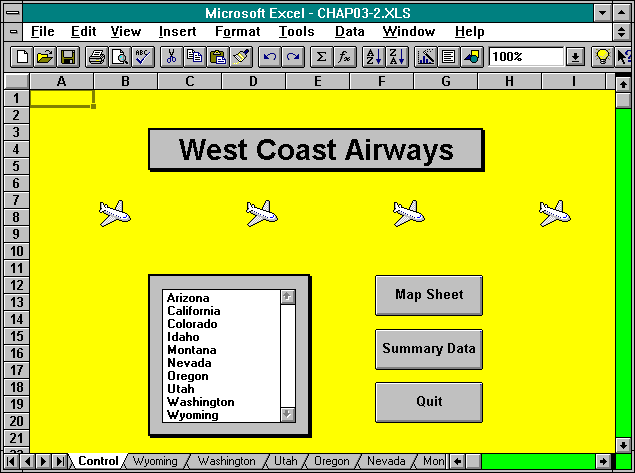
Although you are nearly finished creating the West Coast Airways application, one last task remains. You have probably noticed that many of the Excel artifacts that remind users that they are using a spreadsheet software program still appear in the application. Such artifacts include row and column headings, gridlines on many of the forms, scrollbars, worksheet tabs, and the formula bar at the top and the status bar at the bottom of the work area. Properties of the Window object control some of these artifacts. Properties of the Application object control others. For example, settings for gridlines, row and column headings, tabs, and scrollbars are made through Window properties; settings for the formula bar and status bar display are made through Application properties. You can save Window property settings with a workbook file, but you cannot do so with Application property settings. In addition, some of these Window properties are specific to the Worksheet object, and others are specific to the Workbook object. For example, settings for gridlines and row and column headings are Worksheet specific; settings for scrollbars and tabs are Workbook specific. So to turn off the display of gridlines and row and column headings on all of the forms in the application, you must activate each worksheet and set the appropriate display property for gridlines and row and column headings. You can do this manually by going to each worksheet, choosing the Options command from the Tools menu, and making the appropriate selections from the View tab. The necessary Workbook-specific and Application-specific property settings can be made in the same Options dialog box, but they need be made only one time. However, the SetUpEnvironment macro below will perform all these tasks for you:
Sub SetUpEnvironment()
    Dim WorksheetVar As Worksheet
    For Each WorksheetVar In ActiveWorkbook.Worksheets
        WorksheetVar.Select
        With ActiveWindow
            .DisplayGridlines = False
            .DisplayHeadings = False
        End With
    Next
    With ActiveWindow
        .DisplayHorizontalScrollBar = False
        .DisplayVerticalScrollBar = False
        .DisplayWorkbookTabs = False
    End With
    Application.DisplayFormulaBar = False
    Application.DisplayStatusBar = False
    Worksheets("Control").Activate
End Sub
SetUpEnvironment uses a For-Each-Next loop to set all of the Worksheet-specific Window properties and then uses a With statement on the ActiveWindow to set all of the Workbook-specific Window properties. Last the macro sets the necessary Application-specific properties.
Run the SetUpEnvironment macro. If you save the file, all but the Application-specific property settings are saved with the file and are then restored when the file is opened again. To restore the Application property settings, write an Auto_Open macro that sets the property settings whenever the workbook file is opened.
The Auto_Open macro below sets the Application-specific properties of DisplayStatusBar and DisplayFormulaBar:
Sub Auto_Open()
    Application.DisplayStatusBar = False
    Application.DisplayFormulaBar = False
End Sub
Auto_Open is called automatically when the file is opened. Note that VBA also provides an Auto_Close macro that runs every time a workbook file is closed. After you add the Auto_Open macro, return to the Control form and save the file.
If you would like to review the code in Module1, you can redisplay the worksheet tabs through the Options dialog box, or you can press the Ctrl-PgUp or Ctrl-PgDown keys until Module1 becomes the active sheet. Such key combinations let you move from one sheet to another without using tabs.
Congratulations! You have successfully built the West Coast Airways application. As mentioned, this application suffers from a few flaws that would limit its implementation as a full-fledged information system. If you have mastered the concepts covered in this chapter, however, you are well on your way to building powerful information systems in Excel.
The rest of the chapters in this book cover more advanced topics associated with more complicated Excel objects, including database access, data flow, control of user input, and e-mail integration. Mastering these advanced topics and the more complicated objects in Excel will allow you to transform applications such as West Coast Airways into full-fledged information systems. The discussion of such advanced topics begins with the next chapter, "Building Information Systems with Pivottables and Charts."
This chapter introduced most of Excel's graphical objects and showed you how to manipulate them through VBA to create a simple application. The following list summarizes this chapter's key points: