In the special case of a dataset consisting of only the Measures dimension along the x-axis, the resulting flattened view is typical of the way in which atomic OLAP data is commonly stored in a relational database. This table of granular data is called a fact table. The combination of a fact table and a set of related dimension tables make up a star schema configuration.
For example, consider the MDX statement below (unqualified names are assumed to be unique):
SELECT
   {Sales, Cost} ON COLUMNS,
   CROSSJOIN({USA, Asia}, {Qtr1, Qtr2, Qtr3, Qtr4}} ON ROWS
FROM SalesCube
WHERE ([1991], Computers)
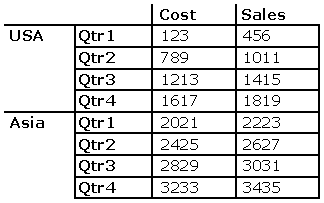
This produces the dataset below:

This yields the flattened rowset:
| [Continents]. [MEMBER_ CAPTION] |
[Countries]. [MEMBER_ CAPTION] |
[Quarters]. [MEMBER_ CAPTION] |
[Measures]. [Cost] |
[Measures]. [Sales] |
| North America | USA | Qtr1 | 123 | 456 |
| North America | USA | Qtr2 | 789 | 1011 |
| North America | USA | Qtr3 | 1213 | 1415 |
| North America | USA | Qtr4 | 1617 | 1819 |
| Asia | NULL | Qtr1 | 2021 | 2223 |
| Asia | NULL | Qtr2 | 2425 | 2627 |
| Asia | NULL | Qtr3 | 2829 | 3031 |
| Asia | NULL | Qtr4 | 3233 | 3435 |
This representation is intuitive and corresponds to the way such data is usually displayed in a tabular view.
This example also illustrates step 2 of the algorithm given in “Flattening Algorithm”: If the DIMENSION PROPERTIES clause is not specified, then it is equivalent to specifying DIMENSION PROPERTIES MEMBER_CAPTION.