Suriya Narayanan
Microsoft SQL Server Technical Note
Volume 4, Number 4
February 1994
Client-server solutions are being implemented at an increasingly rapid rate. More and more mission-critical applications are being downsized from mainframe-based proprietary computing platforms to open, personal computer–based platforms. This has resulted in the widespread use of Microsoft® SQL Server for the Windows NT™ operating system and the creation of very large databases in SQL Server. For certain classes of problems, a conventional design of the database would not give an optimal, high-performance solution. This technical note addresses one such class of problems and discusses an unconventional implementation of the database using the binary data type and bitwise operations available in Microsoft SQL Server.
Say, for example, that a toy retailer wants to implement a database of all the products carried in each store. The retailer must identify and classify the different types of toys carried. Each toy will be assigned a unique number, called toy number. If someone knows the toy number, then he or she can query the database to find out all the information about the toy, such as the manufacturer, the target audience (boys or girls), price, how many are available, and so on. But this is possible only if someone knows the toy number. Given tens of thousands of toys carried by the retailer, it is impossible for anyone to remember the toy number. Nor it is possible to load all the toy numbers in a list box and let the user pick one.
What the retailer needs is a way to classify and describe the toys, so that a person who does not know the toy number can start describing the toy(s) and the database will use the description to find the specific toy(s). Obviously, the more description a person provides, the better the chance that the correct toy will be retrieved. For example, a person can describe a toy as being mostly used by girls between the ages of 3 and 5, having wheels, being battery operated, and manufactured by Acme Toy Company. The system uses this description and lists 20 toys satisfying this description. By further describing the toy, the user can narrow the selected set of toys to just one.
When dealing with tens of thousands of toys, it would be very easy to assign two different toy numbers to the same toy. It would then be possible for the toy to have two different prices, two different inventory levels, and so on. These duplicate sets of data would confuse the retailer. With the new system described here (of maintaining descriptions of the toys), you can enforce uniqueness, not by the toy number, but by its description. If two different toys have identical descriptions, then they must have identical toy numbers. Thus, the new system will not only help users find particular toys more easily, but it will also clean up the toys data considerably, offering several advantages to the business.
Every organization dealing with several different types of products faces the above problem and needs a solution. In fact, in certain industries, such as building products, the problem is even larger in scope. Imagine a building products retail store carrying more than 300,000 products!
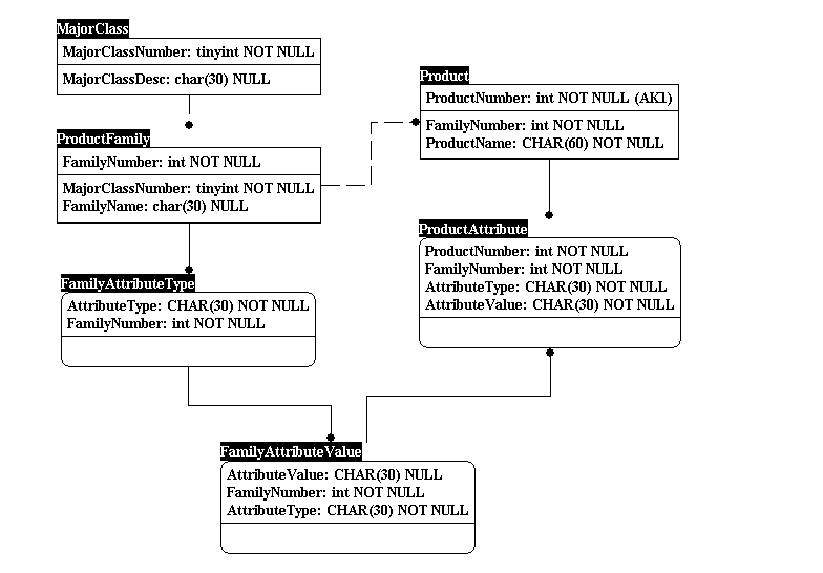
Figure 1 shows the conventional data model for the class of problems described earlier.

Figure 1. Conventional data model
The table MajorClass contains the highest level of classification of products. For example, our toy retailer carries toys, children's books, clothing, furniture, and so on. The MajorClass table will have one row for each of these highest-level products. The next level of classification is the product family. For example, the major class called "children's furniture" can be further classified into several smaller categories, such as cribs, strollers, and bedding. Each such subclassification is identified by a unique number (FamilyNumber), and the table ProductFamily contains all such product families. Within each family, the products are identified further by their properties, or attributes. Each attribute is identified by a unique name, and each attribute type can have many values. For example, the toy Cartoon Truck can belong to the family called Toys Based on Animation. The attribute types Target Age Group and Has Wheels can also be used to describe this toy. The corresponding values of these attribute types might be 7–10 and YES.
Every product belongs to one and only one family and is described by the collection of its attribute types and corresponding values.
Even though the conventional data model truly represents the products and their attributes, it has significant problems. Searching for products using the attribute types and values translates into looking through the ProductAttributes table. This table has one row for each AttributeType–AttributeValue–ProductNumber–FamilyNumber combination. Each row in this table represents only one attribute type and its corresponding value for the given product; it does not represent the entire set of attribute types and values for the product. Given a type Ti and its Value Vi in a family F, the query to select all products looks like this:
Select    ProductAttributes.ProductNumber, ProductName
from      Product, ProductAttributes
where     Product.ProductNumber=ProductAttributes.ProductNumber AND
          ProductFamilyNumber = F AND
          AttributeType = Ti AND
          AttributeValue = Vi
Figure 2. Query to retrieve products having a given attribute type and value
If you have the set of attribute types (T0, T1, T2, . . . TN) and their corresponding values (V0, V1, V2, . . . VN), the query to retrieve all the products having all these attribute types and values is done iteratively, using one attribute type and value at a time. Figure 3 shows the pseudo-query to do this.
Select    AttributeType, AttributeValue, ProductNumber
into      #t1
from      ProductAttributes
where     ProductNumber in
(
          Select    ProductNumber
          from ProductAttributes
          where ProductFamilyNumber = F AND
                AttributeType = T0 AND
                AttributeValue = V0
)

For j = 1 to N
          Select    AttributeType, AttributeValue, ProductNumber
          into #t2
          from #t1
          whereProductNumber in
          (
               Select    ProductNumber
               from #t1
               whereAttributeType = Ti  AND
                    AttributeValue = Vj
           )

          delete from #t1
          insert into #t1 (AttributeType, AttributeValue, ProductNumber)
          select    AttributeType, AttributeValue, ProductNumber
          from    #t2
Next j

select    #t1.ProductNumber, ProductName
from      #t1, Products
where     #t1.ProductNumber = Products.ProductNumber
Figure 3. Query using multiple attribute types and values
The query in Figure 3 uses temporary tables extensively. If we assume that there are 300,000 products, and an average of 10 attribute types and corresponding values per product, the ProductAttributes table will have about 3 million rows. Using one attribute type and one attribute value might select 100,000 out of the 3 million rows. The query in Figure 3 will save these 100,000 rows in the temporary table. In a multiuser situation, each user will be saving 100,000 rows in a separate temporary table, causing an enormous amount of disk writes. Finding the duplicate products (two or more products in the same family having identical attribute types and values) is next to impossible in this data model. Certain other types of queries, such as retrieving all products having the attribute type LENGTH and its corresponding value, any one of the set (10, 12, 14, 16), is very difficult to implement.
The problems with this data model are fundamental in nature. Each row in the ProductAttributes table represents only one attribute type and its value, but the set of attribute types and their values represents the product. The set of attribute types and their values cannot be stored in this table in one row without violating the first normal form.
The only advantage of this data model is that it supports an unlimited number of attribute types per family and an unlimited number of distinct values in each attribute type. In reality, however, such an unlimited number of attribute types and attribute values is rarely used.
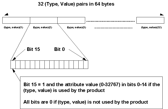
The new, improved data model uses a variation of a technique called hashing to convert the set of attribute types and values into a single value representing the entire collection of attribute types and values. Here is the hashing scheme used to encode all the attribute types and values:
One can create 32 such 2-byte numbers, one for each attribute type–attribute value pair. Concatenating all of them in the order (T0, V0), (T1, V1), (T2, V2), . . . (T31, V31) creates a 64-byte binary number. This large number is the single value representing the collection of attribute types and corresponding values of a product. Figure 4 shows the structure of this 64-byte binary number.

Figure 4. Combining attribute types and values
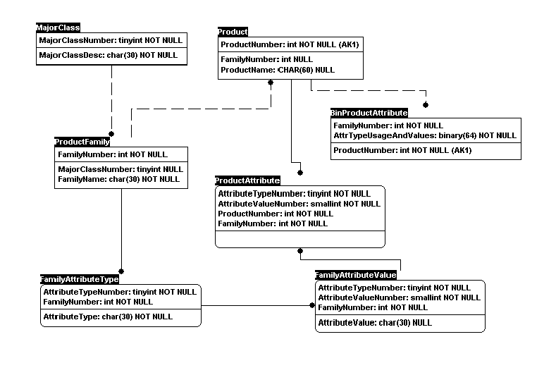
Figure 5 shows the new data model. The table BinProductAttributes contains the encoded attribute types and values of the products. This table has exactly one row for every product. The column AttrTypeUsageAndValues contains all the attribute types and corresponding values in the encoded form. Creating a unique index of the FamilyNumber and the AttrTypeUsageAndValues columns will instantly identify the duplicate products.

Figure 5. New data model
All the attribute types and values are combined to form the binary key for the product. This can be done in SQL Server itself, using the bitwise and substring operations on the binary column. However, a more natural implementation of this would be in C, where the bitwise operations can be done more easily. The binary key also can be represented as an array of bytes in C, resulting in an easier manipulation of the individual bytes in the binary key. The algorithm can be implemented as extended stored procedures in SQL Server for Windows NT. You need two stored procedures, xp_EncodeAttrTypeValue and xp_DecodeAttrTypeValue, to encode the attribute types and values into the binary key and to decode the binary key into individual attribute types and values, respectively.
The new model contains all the attribute types and values encoded into one binary key. Using attribute types and values to query for products will require doing a partial match on the binary column AttrTypeUsageAndValues using bitwise operations. For example, say you are searching for all the products with a LENGTH of 10 feet. The AttributeTypeNumber for the Attribute LENGTH is, for example, 14, and the AttributeValueNumber for the value 10 feet is, for example, 346. Then you need to include all the products for which bytes 27 and 28 of the AttrTypeUsageAndValues column (which corresponds to the fourteenth attribute type–attribute value pair) contain the value 346 in bits 0 through 14, and bit 15 is 1. This type of search is accomplished using bitwise operations.
The extended stored procedure xp_EncodeAttrTypeValue can also generate a mask—a 64-byte bit pattern, which will have 1s on all the bits for all the attribute types and values we know and 0s for remaining bits. This extended stored procedure takes 32 attribute type numbers and 32 corresponding attribute value numbers as input parameters and returns the 64-byte key generated and the 64-byte key mask as output. If a certain attribute type and value is not used, a special value (for example, –1) is passed instead of the attribute type number, and the generated key will have 0s in its corresponding position. For the above example, the mask will have 0xFFFF in bytes 27 and 28, and 0s in the remaining bytes. SQL Server requires that one of the operands in a bitwise operation be a tinyint, smallint, int, or a bit. Therefore, the mask and the binary key cannot be bitwise ANDed directly. They must be split into parts and each part ANDed separately. Figure 6 shows the pseudo-query.
declare     @key binary(64), @keymask binary(64)

/* @ts and @vs are the attribute types and corresponding values respectively */

execute   master.dbo.xp_EncodeAttrTypeValue
            @t01, @v01, @t02, @v02, @t03, @v03, @t04, @v04,
            @t05, @v05, @t06, @v06, @t07, @v07, @t08, @v08,
            @t09, @v09, @t10, @v10, @t11, @v11, @t12, @v12,
            @t13, @v13, @t14, @v14, @t15, @v15, @t16, @v16,
            @t17, @v17, @t18, @v18, @t19, @v19, @t20, @v20,
            @t21, @v21, @t22, @v22, @t23, @v23, @t24, @v24,
            @t25, @v25, @t26, @v26, @t27, @v27, @t28, @v28,
            @t29, @v29, @t30, @v30, @t31, @v31, @t32, @v32,
            @EncodedKey = @key OUTPUT,     /* Key */
            @EncodedKeyMask = @keymask OUTPUT  /* Mask */

select  Product.ProductNumber, Product.ProductName
from    BinProductAttributes, Product
where   BinProductAttributes.ProductFamilyNumber = @family AND
        BinProductAttributes.ProductNumber =
        Product.ProductNumber AND
        AttrTypeUsageAndValues >= @key AND

/* Bitwise AND the generated key and the key mask in parts */

        convert(int, substring(AttrTypeUsageAndValues, 1, 4)) &
            substring(@keymask, 1, 4) = substring(@key, 1, 4) AND
        convert(int, substring(AttrTypeUsageAndValues, 5, 4)) &
            substring(@keymask, 5, 4) = substring(@key, 5, 4) AND
        convert(int, substring(AttrTypeUsageAndValues, 9, 4)) &
            substring(@keymask, 9, 4) = substring(@key, 9, 4) AND
        convert(int, substring(AttrTypeUsageAndValues, 13, 4)) &
            substring(@keymask, 13, 4) = substring(@key, 13, 4) AND
        convert(int, substring(AttrTypeUsageAndValues, 17, 4)) &
            substring(@keymask, 17, 4) = substring(@key, 17, 4) AND
        convert(int, substring(AttrTypeUsageAndValues, 21, 4)) &
            substring(@keymask, 21, 4) = substring(@key, 21, 4) AND
        convert(int, substring(AttrTypeUsageAndValues, 25, 4)) &
            substring(@keymask, 25, 4) = substring(@key, 25, 4) AND
        convert(int, substring(AttrTypeUsageAndValues, 29, 4)) &
            substring(@keymask, 29, 4) = substring(@key, 29, 4) AND
        convert(int, substring(AttrTypeUsageAndValues, 33, 4)) &
            substring(@keymask, 33, 4) = substring(@key, 33, 4) AND
        convert(int, substring(AttrTypeUsageAndValues, 37, 4)) &
            substring(@keymask, 37, 4) = substring(@key, 37, 4) AND
        convert(int, substring(AttrTypeUsageAndValues, 41, 4)) &
            substring(@keymask, 41, 4) = substring(@key, 41, 4) AND
        convert(int, substring(AttrTypeUsageAndValues, 45, 4)) &
            substring(@keymask, 45, 4) = substring(@key, 45, 4) AND
        convert(int, substring(AttrTypeUsageAndValues, 49, 4)) &
            substring(@keymask, 49, 4) = substring(@key, 49, 4) AND
        convert(int, substring(AttrTypeUsageAndValues, 53, 4)) &
            substring(@keymask, 53, 4) = substring(@key, 53, 4) AND
        convert(int, substring(AttrTypeUsageAndValues, 57, 4)) &
            substring(@keymask, 57, 4) = substring(@key, 57, 4) AND
        convert(int, substring(AttrTypeUsageAndValues, 61, 4)) &
            substring(@keymask, 61, 4) = substring(@key, 61, 4)
Figure 6. Product selection query in the new data model
The binary key generated by the extended stored procedure also has an interesting use. For example, if you specify only two attribute types and values, the generated key contains the attribute values in their corresponding positions and 0s everywhere else. If we keep the table sorted in the ascending order of the FamilyNumber and AttrTypeUsageAndValues columns (by creating a clustered index on the columns), then all the products in the same family with only the given two attribute types and values must occur before all the products using other type–value pairs in addition to the given two type–value pairs. Therefore, the generated key also has ordering information with respect to all other keys in the table. The WHERE clause would include a search for a key greater than or equal to the generated key. Every key in the table following the first key greater than or equal to the generated key must be bitwise ANDed with the key mask. The binary key is generated by combining the sequence of type–value pairs (T0, V0), (T1, V1), (T2, V2), . . . (T31, V31) in that order. Because binary columns are compared left to right, specifying type–value pairs from the beginning of the sequence, such as (T0, V0), (T1, V1), will generate keys with the leftmost bytes nonzero, and therefore will improve the selectivity of the rows, when used in the WHERE clause.
Both the conventional and the new data models were implemented and the response times of the products-selection query measured. The query operated several orders of magnitude faster in the new model. In the conventional model, the bottleneck was the disk writes and reads. Every additional attribute type and value generates extra writes and reads from temporary tables. As a result, the more attribute types and values specified, the slower the query will run. In a multiuser scenario, even more temporary tables are created (a separate set of temporary tables for each user), increasing the disk writes and reads, resulting in even slower performance. The CPU utilization curve in the Performance Monitor has very steep peaks and valleys. The valleys in the curve correspond to the times when SQL Server was performing much disk input/output.
In the new model, the query does not use any temporary tables and therefore does not generate any extra disk writes and reads. The response time depends on how many rows have to be bitwise ANDed with the key mask. This is acceptable because the CPU operations are several orders of magnitude faster than disk operations. The CPU utilization curve in the Performance Monitor appears more evenly spread out. The CPU utilization stays constant for short periods of time, corresponding to the times when large scale bitwise operations are done. The bottleneck in the new model is the CPU. In a multiuser scenario, more and more queries will demand that the CPU perform bitwise operations. Using a faster CPU or an SMP (symmetric multiprocessing) computer will help improve performance.
Hussey, Peter. "Extended Stored Procedures and Open Data Services: An Overview." MSDN Library Archive, Conference and Seminar Papers.
Moffatt, Christopher. "Designing Client-Server Applications for Enterprise Database Connectivity." MSDN Library, Technical Articles.
Moffatt, Christopher. "Microsoft SQL Server Network Integration Architecture." MSDN Library, Technical Articles.
"Query Optimization Techniques." MSDN Library, Technical Articles.
Schroeder, Gary. "Backup and Recovery Guidelines for Microsoft SQL Server." MSDN Library, Technical Articles.
To receive more information about Microsoft SQL Server or to have other technical notes faxed to you, call Microsoft Developer Services FAX Request at (206) 635-2222.