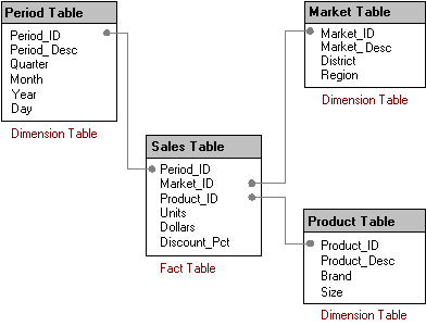
Databases designed for decision support, particularly data warehouses and data marts, often have very different table structures than OLTP databases. A common approach is to implement a star schema, a type of database schema designed to allow a user to intuitively navigate information in the database, as well as to provide better performance for large, ad hoc queries.
A star schema begins with the observation that information can be classified into facts, the numeric data that is the core of what is being analyzed, and dimensions, the attributes of facts. Examples of facts include sales, units, budgets, and forecasts. Examples of dimensions include geography, time, product, and sales channel. Users often express their queries by saying “I want to look at these facts by these dimensions,” or “I want to look at sales and units sold by quarter.”
A star schema takes advantage of this observation by organizing data into a central fact table and surrounding dimension tables.

Microsoft SQL Server 7.0 has several techniques for optimizing queries against star schemas. The query processor automatically recognizes these queries and applies any and all of the techniques presented here, as well as combinations of these techniques. It is important to understand that the choice of which technique to apply is entirely cost-based; no hints are required to force these optimizations.
The tables in a star schema do not contain equal numbers of records. Typically, the fact table has many more records. This difference becomes important in many of the query optimization techniques.
A straightforward execution strategy is to read the entire fact table and join it in turn to each of the dimension tables. If no filter conditions are specified in the query, this can be a reasonable strategy. However, when filter conditions are present, the star query optimizations avoid having to read the entire fact table by taking full advantage of indexes.
Because dimension tables typically have fewer records than the fact table, it can make sense to compute the Cartesian product and use the result to view fact table rows in a multicolumn index.
For example, assume that the sales (fact) table has 10 million rows, the period table has 20 rows, the market table has 5 rows, and the product table has 200 rows. Also assume that a user generates this query using a front-end tool:
SELECT        sales.market_id, period.period_id, sum(units), sum(dollars)

FROM        sales, period, market

WHERE        period.period_id = sales.period_id and

                sales.market_id = market.market_id and

                period.period_Desc in (‘Period2’,’Period3’,’Period4’,’Period5’)

                and market.market_Desc in (‘Market1’,’Market2’)

GROUP BY sales.market_id, period.period_id
A simple approach is to join the period table to the sales table. Assuming an even distribution of data, the input is 10 million rows, the output is 4/20 (4 periods out of a possible 20), or 2 million rows. This can be done using a hash join or merge join and involves reading the entire 10 million rows in the fact table or retrieving 2 million rows through index lookups, whichever costs less. This partial result is then joined to the reduced market table to produce 800K rows of output, which are finally aggregated.
If there is a multicolumn index on the fact table (for example, on period_id or market_id) the Cartesian product strategy can be used. Because there are 4 rows selected from the period table and 2 rows from the market table, the Cartesian product is 8 rows. These eight combinations of values are used to look up the resulting 800K rows of output. Multicolumn indexes used this way are sometimes called star indexes.
If the joins to the fact table occur on fields other than those contained in a composite index, the query optimizer can use other indexes and reduce the number of rows read from the fact table by performing an intersection of the qualifying rows from joins to each dimension table.
For example, if period_id or product_id is selected, the query optimizer cannot use the composite index because the two fields of interest are not a leading subset of the index. However, if there are separate single-column indexes on period_id and product_id, the query optimizer may choose a join between the period table and the sales table (retrieving 2 million index entries) and, separately, a join between the product table and the sales table (retrieving 4 million index entries). In both cases, the optimizer will do the join using an index; thus, the two preliminary joins compute sets of record IDs for the sales table but not full rows of the sales table. Before retrieving the actual rows in the sales table (the most expensive process), an intersection of the two sets is computed to determine the qualifying rows. Only rows that satisfy both joins are included in this intermediate result of 800K rows and only these rows are actually read from the sales table.
Occasionally, semi-join reduction can be combined with Cartesian products and composite indexes. For example, if you select from three dimension tables, where two of the three tables are the initial fields of a composite index but the third dimension has a separate index, the query optimizer can use Cartesian products to satisfy the first two joins, use semi-joins to satisfy the third join, and then combine the results.
Several factors influence the effectiveness of these techniques. These factors include the size of the indexes to be used compared to the base table, and whether the set of indexes used covers all the columns required by the query, obviating the need to look up rows in the base table. These factors are taken into account by the query optimizer, which will choose the least expensive plan.
If that plan is more expensive than the cost threshold for parallelism, all required operations, including scans, joins, intersection, and row fetching, can be executed by multiple threads in parallel.