INDEX (Reference Form)

Returns the reference of the cell at the intersection of a particular row and column. If the reference is made up of nonadjacent selections, you can pick the selection to look in.

The INDEX function has two syntax forms: array and reference. The array form always returns a value or an array of values; the reference form always returns a reference.

Syntax 2

Reference form

INDEX(reference,row_num,column_num,area_num)

Reference   is a reference to one or more cell ranges.

• If you are entering a nonadjacent selection for reference, enclose reference in parentheses. For an example of using INDEX with a nonadjacent selection, see the fifth example following.
• If each area in reference contains only one row or column, the row_num or column_num argument, respectively, is optional. For example, for a single row reference, use INDEX(reference,,column_num).

Row_num   is the number of the row in reference from which to return a reference.

Column_num   is the number of the column in reference from which to return a reference.

Area_num   selects a range in reference from which to return the intersection of row_num and column_num. The first area selected or entered is numbered 1, the second is 2, and so on. If area_num is omitted, INDEX uses area 1.

For example, if reference describes the cells (A1:B4,D1:E4,G1:H4), then area_num 1 is the range A1:B4, area_num 2 is the range D1:E4, and area_num 3 is the range G1:H4.

After reference and area_num have selected a particular range, row_num and column_num select a particular cell: row_num 1 is the first row in the range, column_num 1 is the first column, and so on. The reference returned by INDEX is the intersection of row_num and column_num.

If you set row_num or column_num to 0 (zero), INDEX returns the reference for the entire column or row, respectively.

Remarks

• Row_num, column_num, and area_num must point to a cell within reference; otherwise, INDEX returns the #REF! error value. If row_num and column_num are omitted, INDEX returns the area in reference specified by area_num.
• The result of the INDEX function is a reference and is interpreted as such by other formulas. Depending on the formula, the return value of INDEX may be used as a reference or as a value. For example, the formula CELL("width",INDEX(A1:B2,1,2)) is equivalent to CELL("width",B1). The CELL function uses the return value of INDEX as a cell reference. On the other hand, a formula such as 2*INDEX(A1:B2,1,2) translates the return value of INDEX into the number in cell B1.

Examples

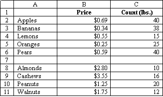
On the following worksheet, the range A2:C6 is named Fruit, the range A8:C11 is named Nuts, and the range A1:C11 is named Stock.

INDEX(Fruit,2,3) equals the reference C3, containing 38

INDEX((A1:C6,A8:C11),2,2,2) equals the reference B9, containing $3.55

SUM(INDEX(Stock,0,3,1)) equals SUM(C1:C11) equals 216

SUM(B2:INDEX(Fruit,5,2)) equals SUM(B2:B6) equals 2.42