LINEST

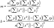
Calculates the statistics for a line by using the "least squares" method to calculate a straight line that best fits your data, and returns an array that describes the line. Because this function returns an array of values, it must be entered as an array formula.

The equation for the line is:

y = mx + b or y = m₁x₁ + m₂x₂ + ^... + b (if there are multiple ranges of x-values)

where the dependent y-value is a function of the independent x-values. The m-values are coefficients corresponding to each x-value, and b is a constant value. Note that y, x, and m can be vectors. The array that LINEST returns is {m_n,m_n-1, ...,m₁,b}. LINEST can also return additional regression statistics.

Syntax

LINEST(known_y's,known_x's,const,stats)

Known_y's   is the set of y-values you already know in the relationship y = mx + b.

• If the array known_y's is in a single column, then each column of known_x's is interpreted as a separate variable.
• If the array known_y's is in a single row, then each row of known_x's is interpreted as a separate variable.

Known_x's   is an optional set of x-values that you may already know in the relationship y = mx + b.

• The array known_x's can include one or more sets of variables. If only one variable is used, known_y's and known_x's can be ranges of any shape, as long as they have equal dimensions. If more than one variable is used, known_y's must be a vector (that is, a range with a height of one row or a width of one column).
• If known_x's is omitted, it is assumed to be the array {1,2,3, ...} that is the same size as known_y's.

Const   is a logical value specifying whether to force the constant b to equal 0.

• If const is TRUE or omitted, b is calculated normally.
• If const is FALSE, b is set equal to 0 and the m-values are adjusted to fit y = mx.

Stats   is a logical value specifying whether to return additional regression statistics.

• If stats is TRUE, LINEST returns the additional regression statistics, so the returned array is {m_n,m_n-1, ...,m_1,b;se_n,se_n-1, ...,se₁,se_b;r2,se_y;F,df;ss_reg,ss_resid}.
• If stats is FALSE or omitted, LINEST returns only the m-coefficients and the constant b.

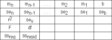
The additional regression statistics are as follows.

The following illustration shows the order in which the additional regression statistics are returned.

Remarks

• You can describe any straight line with the slope and the y-intercept:

  Slope (m):
  To find the slope of a line, often written as m, take two points on the line, (x₁,y₁) and (x₂,y₂); the slope is equal to (y₂ - y₁)/(x₂ - x₁).

  Y-intercept (b):
  The y-intercept of a line, often written as b, is the value of y at the point where the line crosses the y-axis.

  The equation of a straight line is y = mx + b. Once you know the values of m and b, you can calculate any point on the line by plugging the y- or x-value into that equation. You can also use the TREND function. For more information, see TREND.

• When you have only one independent x-variable, you can obtain the slope and y-intercept values directly by using the following formulas:

  Slope:
  INDEX(LINEST(known_y's,known_x's),1)

  Y-intercept:
  INDEX(LINEST(known_y's,known_x's),2)

• The accuracy of the line calculated by LINEST depends on the degree of scatter in your data. The more linear the data, the more accurate the LINEST model. LINEST uses the method of least squares for determining the best fit for the data. When you have only one independent x-variable, the calculations for m and b are based on the following formulas:

  

• The line- and curve-fitting functions LINEST and LOGEST can calculate the best straight line or exponential curve that fits your data. However, you have to decide which of the two results best fits your data. You can calculate TREND(known_y's,known_x's) for a straight line, or GROWTH(known_y's, known_x's) for an exponential curve. These functions, without the new_x's argument, return an array of y-values predicted along that line or curve at your actual data points. You can then compare the predicted values with the actual values. You may want to chart them both for a visual comparison.
• In regression analysis, Microsoft Excel calculates for each point the squared difference between the y-value estimated for that point and its actual y-value. The sum of these squared differences is called the residual sum of squares. Microsoft Excel then calculates the sum of the squared differences between the actual y-values and the average of the y-values, which is called the total sum of squares (regression sum of squares + residual sum of squares). The smaller the residual sum of squares is, compared with the total sum of squares, the larger the value of the coefficient of determination, r², which is an indicator of how well the equation resulting from the regression analysis explains the relationship among the variables.
• Formulas that return arrays must be entered as array formulas.
• When entering an array constant such as known_x's as an argument, use commas to separate values in the same row and semicolons to separate rows. Separator characters may be different depending on your country settings.
• Note that the y-values predicted by the regression equation may not be valid if they are outside the range of the y-values you used to determine the equation.

Example 1   Slope and Y-Intercept

LINEST({1,9,5,7},{0,4,2,3}) equals {2,1}, the slope = 2 and y-intercept = 1

Example 2   Simple Linear Regression

Suppose a small business has sales of $3,100, $4,500, $4,400, $5,400, $7,500, and $8,100 during the first six months of the fiscal year. Assuming that the values are entered in the range B2:B7, respectively, you can use the following simple linear regression model to estimate sales for the ninth month.

SUM(LINEST(B2:B7)*{9,1}) equals SUM({1000,2000}*{9,1}) equals $11,000

In general, SUM({m,b}*{x,1}) equals mx + b, the estimated y-value for a given x-value. You can also use the TREND function.

Example 3   Multiple Linear Regression

Suppose a commercial developer is considering purchasing a group of small office buildings in an established business district.

The developer can use multiple linear regression analysis to estimate the value of an office building in a given area based on the following variables.

This example assumes that a straight-line relationship exists between each independent variable (x₁, x₂, x₃, and x₄) and the dependent variable (y), the value of office buildings in the area.

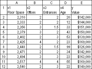
The developer randomly chooses a sample of 11 office buildings from a possible 1,500 office buildings and obtains the following data.

"Half an entrance" means an entrance for deliveries only. When entered as an array, the following formula:

LINEST(E2:E12,A2:D12,TRUE,TRUE)

returns the following output.

The multiple regression equation, y = m₁*x₁ + m₂*x₂ + m₃*x₃ + m₄*x₄ + b, can now be obtained using the values from row 14:

y = 27.64*x₁ + 12,530*x₂ + 2,553*x₃+ 234.24*x₄ + 52,318

The developer can now estimate the assessed value of an office building in the same area that has 2,500 square feet, three offices, and two entrances and is 25 years old, by using the following equation:

y = 27.64*2500 + 12530*3 + 2553*2 - 234.24*25 + 52318 = $158,261

You can also use the TREND function to calculate this value. For more information, see TREND.

Example 4   Using The F And R2 Statistics

In the previous example, the coefficient of determination, or r², is 0.99675 (see cell A16 in the output for LINEST), which would indicate a strong relationship between the independent variables and the sale price. You can use the F statistic to determine whether these results, with such a high r² value, occurred by chance.

Assume for the moment that in fact there is no relationship among the variables, but that you have drawn a rare sample of 11 office buildings that causes the statistical analysis to demonstrate a strong relationship. The term "Alpha" is used for the probability of erroneously concluding that there is a relationship.

There is a relationship among the variables if the F-observed statistic is greater than the F-critical value. The F-critical value can be obtained by referring to a table of F-critical values in many statistics textbooks. To read the table, assume a single-tailed test, use an Alpha value of 0.05, and for the degrees of freedom (abbreviated in most tables as v1 and v2), use v1 = k = 4 and v2 = n - (k + 1) = 11 - (4 + 1) = 6, where k is the number of variables in the regression analysis and n is the number of data points. The F-critical value is 4.53.

The F-observed value is 459.753674 (cell A17), which is substantially greater than the F-critical value of 4.53. Therefore, the regression equation is useful in predicting the assessed value of office buildings in this area.

Example 5   Calculating The T-Statistics

Another hypothesis test will determine whether each slope coefficient is useful in estimating the assessed value of an office building in example 3. For example, to test the age coefficient for statistical significance, divide -234.24 (age slope coefficient) by 13.268 (the estimated standard error of age coefficients in cell A15). The following is the t-observed value:

t = m₄ ÷ se₄ = -234.24 ÷ 13.268 = -17.7

If you consult a table in a statistics manual, you will find that t-critical, single tail, with 6 degrees of freedom and Alpha = 0.05 is 1.94. Because the absolute value of t, 17.7, is greater than 1.94, age is an important variable when estimating the assessed value of an office building. Each of the other independent variables can be tested for statistical significance in a similar manner. The following are the t-observed values for each of the independent variables.

These values all have an absolute value greater than 1.94; therefore, all the variables used in the regression equation are useful in predicting the assessed value of office buildings in this area.