Recursion: The Good, the Bad, and the Ugly

Rod Stephens

In this month's column, Rod discusses recursion, a powerful technique for breaking large problems into small ones. Like most other powerful techniques, recursion is subject to abuse, so Rod gives some good and bad examples of recursion and even shows how to remove recursion when necessary.

Recursion occurs when a function or subroutine calls itself. Programmers often break large problems into smaller pieces, some of which call themselves recursively. The recursive subroutine calls break the pieces into even smaller pieces and call the routine again to handle them. The routine calls itself again and again, breaking the problem into smaller and smaller pieces until they reach a manageable size. At that point, the routine solves the small pieces that make up the larger problem. [Raise your hand if your first introduction to recursion was coding the Tower of Hanoi. -- Ed.]

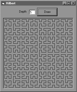
Recursion is a powerful technique, and some recursive routines perform remarkable computations with surprisingly little code. The Hilbert curve routine described near the end of this article draws curves of amazing complexity with just seven lines of code.

To use recursion, you need to think in terms of breaking a problem into pieces that are similar to the original problem but smaller. This is a bit backwards from the way people normally think about breaking up large problems. Usually people think in terms of performing a series of steps one after another in order to accomplish a task. For example, suppose you need to paint a fence. You'd probably start at one end and paint each board in order until you'd reached the other end of the fence.

To recursively paint the fence, you might subdivide the fence into its left and right halves and then recursively paint the two halves. You would then recursively subdivide each half into quarters, each quarter into eighths, and so on until you were considering pieces of fence that contained a single board. At that point, you'd paint the single boards and be finished. I realize this example is silly; it would take you longer to jump back and forth to paint a fence recursively than it would to just start at one side and work across to the other -- you'd be better served borrowing a page from Tom Sawyer's playbook -- but in computer programs, there are many good examples of recursion.

The good
The eighteenth-century mathematician Euler discovered a recursive method for finding greatest common divisors. The greatest common divisor (GCD) of two numbers is the largest integer that evenly divides the two numbers. For example, GCD(12, 20) = 4 because 4 is the largest integer that divides 12 and 20 evenly.

The fact Euler discovered is:

 If A divides B evenly, GCD(A, B) = A. 
 Otherwise GCD(A, B) = GCD(B Mod A, A) 


This leads to a naturally recursive algorithm for finding greatest common divisors:

 Public Function GCD(ByVal A As Long, ByVal B As Long)_ 
    As Long 
 Dim b_mod_a As Long 
    b_mod_a = B Mod A 
    If b_mod_a = 0 Then 
       GCD = A 
    Else 
       GCD = GCD(b_mod_a, A) 
    End If 
 End Function 


To see how this works, you can follow the steps the GCD function takes to calculate a greatest common divisor. Suppose you call this function to calculate GCD(112, 210):

 GCD(112, 210)  = GCD(210 Mod 112, 112)  = 
 GCD(98, 112)   = GCD(112 Mod 98, 98)    = 
 GCD(14, 98) 


At this point, the function stops because 14 divides 98 evenly 7 times. That means GCD(112, 210) = 14. You can verify this yourself because 210/14 = 15 and 112/14 = 8. The values 15 and 8 have no common divisors, so 14 is the largest number that evenly divides 112 and 210. Figuring out how quickly the GCD function works is a little tricky. The key is to prove that the second parameter B to the recursive GCD calls shrinks by a factor of at least 1/2 every two times the function calls itself.

Assume that B is originally larger than A. If it's not, you can verify that the first call to GCD switches the order of the parameters and calls GCD again with the values of A and B swapped. After that, B is always larger.

The next call to the function calculates GCD(B Mod A, A). If A _ B/2, then the second parameter in this first recursive call to GCD is already less than or equal to B/2. The second parameter has decreased by a factor of at least one half, and that's all we need to show.

Suppose that isn't the case. In other words, A > B/2 in the original call to GCD(A, B). The next call is GCD(B Mod A, A). Because A > B/2, A divides into B once with a remainder of B - A. That means B Mod A = B A, so the first recursive call to GCD is equivalent to GCD(B - A, A).

The second call to the function computes GCD(A Mod (B - A), B - A). Because we're assuming that A > B/2, the value B - A < B/2. Since B - A is the second parameter in this function call, this shows that the second parameter in the second recursive call to GCD is no more than 1/2 times the original value of B.

All this means that the value for B passed into the GCD function shrinks by a factor of at least 1/2 every two times the function calls itself. Since the recursion must stop when the value for B reaches 1, the function can call itself at most 2 * Log2(B) times. That makes this a very fast routine. For example, if B is on the order of one million, the function can call itself about 2 * Log2(B), or 40 times. In practice, the function is usually called far fewer times that this to find the GCD of even large numbers.

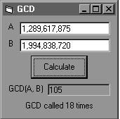
The GCD program, shown in Figure 1 , demonstrates the recursive GDC algorithm. In this example, the function called itself only 18 times to determine that GCD(1,289,617,875, 1,994,838,720) = 105.


The bad
Recursion isn't always the best solution, even when you can figure out how to apply it. For example, Fibonacci numbers have a naturally recursive definition:

 Fibo(0) = 0 
 Fibo(1) = 1 
 Fibo(N) = Fibo(N - 1) + Fibo(N - 2) for N > 1 


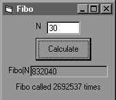
Table 1 shows the values of the first several Fibonacci numbers. The values grow extremely quickly when N is large. For example, Fibo(30) = 832,040.

N 0 1 2 3 4 5 6 7 8 9 10
Fibo(N) 0 1 1 2 3 5 8 13 21 34 55

Table 1: Fibonacci numbers.

The recursive definition of the Fibonacci numbers leads to the following simple recursive function:

 Public Function Fibo(ByVal N As Integer) As Double 
     If N <= 1 Then 
         Fibo = N 
     Else 
         Fibo = Fibo(N - 1) + Fibo(N - 2) 
     End If 
 End Function 


Program Fibo, shown in Figure 2 , demonstrates this algorithm. In addition to calculating Fibonacci numbers, the program displays the number of times the Fibo function was executed. In this example, the function was called more than 2.6 million times to calculate the 30th Fibonacci number. As you might imagine, making all those recursive function calls takes the program a long time.

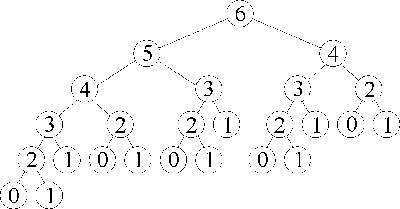
The reason this routine takes so long is that it recalculates a huge number of intermediate values. To compute Fibo(N), the function calls itself with parameters N - 1 and N - 2. To calculate Fibo(N - 1), the routine must calculate Fibo(N - 2) and Fibo(N - 3). Here the value Fibo(N - 2) is calculated twice.


Figure 3 illustrates the function calls used by the Fibo function to calculate Fibo(6). Each number represents a Fibonacci value. Nodes are connected to indicate the intermediate values they must calculate. For example, the root node 6 is connected to nodes labeled 5 and 4 to indicate that the function must calculate Fibo(5) and Fibo(4) to calculate Fibo(6).


Looking at Figure 3 , you can see all of the repeated calculations. The values Fibo(0) and Fibo(1), for example, occur a total of 13 times. In fact, it can be shown that in calculating Fibo(N), the function calculates Fibo(0) and Fibo(1) a total of Fibo(N + 1) times. You can verify this in Figure 3. To calculate Fibo(6), the program evaluates Fibo(0) and Fibo(1) a total of Fibo(6 + 1) = 13 times.


For larger values of N, Fibo(N) grows extremely quickly. For example, Fibo(31) = 1,346,269. That means to calculate Fibo(30), the program recalculates Fibo(0) and Fibo(1) more than 1.3 million times. It's in calculating and recalculating all of these intermediate values that the program spends all of its time.

This is an example of a bad use for recursion. Recursion lets the Fibo function break its calculation into two smaller problems, but the two problems have a lot of overlap. They don't share the work very well and, in fact, duplicate some of each other's efforts. To prevent this wasted duplication, you need to rethink the definition of the Fibonacci numbers. The recursive function uses a top-down approach. While the input number is greater than 1, the function breaks the problem into two smaller problems and solves them recursively.

An alternative bottom-up strategy starts with the known values for Fibo(0) and Fibo(1). It combines those values to produce Fibo(2). It then combines Fibo(1) and Fibo(2) to calculate Fibo(3). It continues combining smaller values to build bigger values until it reaches the value of Fibo(N) that it needs. Instead of breaking a big problem into small pieces, it starts with small values and combines them to calculate bigger values.

Program Fibo2 uses the following code to compute Fibonacci numbers. Although Fibonacci numbers are integers, this code performs its calculations using doubles so it can compute approximate values for very large Fibonacci numbers.

 Public Function Fibo(ByVal N As Integer) As Double 
 Dim fibo_i_minus_2 As Double 
 Dim fibo_i_minus_1 As Double 
 Dim fibo_i As Double 
 Dim i As Integer 
    ' Set Fibo(i) and Fibo(i - 1) for i = 1. 
    fibo_i_minus_1 = 0 
    fibo_i = 1 
    ' Calculate larger values for Fibo(i). 
    For i = 2 To N 
       fibo_i_minus_2 = fibo_i_minus_1 
       fibo_i_minus_1 = fibo_i 
       fibo_i = fibo_i_minus_1 + fibo_i_minus_2 
    Next i 
    Fibo = fibo_i 
 End Function 


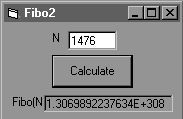
Figure 4 shows program Fibo2 calculating Fibo(1476), the largest value it can compute without causing a double precision overflow. While program Fibo takes more than 10 seconds to calculate Fibo(30) on a (vintage?) 133 MHz Pentium, program Fibo2 takes almost no time to calculate Fibo(1476).


The ugly
Sometimes it's useful to rewrite a recursive algorithm in a non-recursive way. Rewriting the Fibo function saves it from a huge amount of duplicated effort. Some programming languages don't allow recursion, so you need to implement all functions non-recursively in those languages. Early versions of VB also had a limited stack. [In fact, all it takes to do recursion is the ability to pass parameters on the stack and create local variables, something almost all "modern" programming languages let you do. -- Ed.] A recursive routine could only call itself a certain number of times before exhausting the stack space and crashing. The exact depth of recursion possible depended on the amount of memory available and on the amount of memory used by each function call.

It's not always easy to rewrite an algorithm non-recursively, but it's always possible. For an example that's more complex than the Fibo function, consider the Hilbert program, the results of which are shown in Figure 5 . The Hilbert subroutine is multiply recursive, calling itself in four different places.


 Private Sub Hilbert(ByVal depth As Integer, ByVal dx _ 
    As Single, ByVal dy As Single) 
    If depth > 1 Then Hilbert depth - 1, dy, dx 
    picHilbert.Line -Step(dx, dy) 
    If depth > 1 Then Hilbert depth - 1, dx, dy 
    picHilbert.Line -Step(dy, dx) 
    If depth > 1 Then Hilbert depth - 1, dx, dy 
    picHilbert.Line -Step(-dx, -dy) 
    If depth > 1 Then Hilbert depth - 1, -dy, -dx 
 End Sub 


Rewriting this routine from scratch without recursion could be quite difficult because it doesn't have simple top-down and bottom-up versions for you to use. Fortunately, there's a methodical system for converting recursive algorithms into non-recursive ones.

The idea is to simulate the steps the computer takes to perform recursion. Before calling the recursive routine, the computer saves the information it will need to continue running after the recursive call finishes. It saves any variable values that it will need later. It also saves its current location in the code so it knows where to continue execution later. The line of code the computer is currently executing is stored in a program counter, or pc for short.

To mimic these steps in VB, start by labeling all of the places the program will need to resume execution in the routine. This includes the beginning of the routine and each of the lines that follow a recursion. (The labels in the following code are to help you keep track of where the program should continue execution and aren't actually part of the VB code.)

 Private Sub Hilbert(ByVal depth As Integer, ByVal dx _ 
    As Single, ByVal dy As Single) 
 1  If depth > 1 Then Hilbert depth - 1, dy, dx 
 2  picHilbert.Line -Step(dx, dy) 
    If depth > 1 Then Hilbert depth - 1, dx, dy 
 3  picHilbert.Line -Step(dy, dx) 
    If depth > 1 Then Hilbert depth - 1, dx, dy 
 4  picHilbert.Line -Step(-dx, -dy) 
    If depth > 1 Then Hilbert depth - 1, -dy, -dx 
 End Sub 


Next, create a collection for each value the program needs to save before simulating a recursion. This includes any variables the routine will need after the recursion and the program counter. The saved program counter will tell the program where to continue execution after a recursion finishes.

You can make saving and restoring values easier by writing SaveValues and RestoreValues subroutines. These routines take values to save or restore as parameters and then add or remove them from the collections.

To rewrite the recursive routine, use an integer variable pc to keep track of the code segment that the routine should be executing. Place all the code inside a big While loop that contains a Select statement. The cases in the Select statement should be the labels used to divide the code earlier. Each time it passes through the While loop, the Select statement makes the program execute the code indicated by the pc variable. Listing 1 shows the general structure of the non-recursive Hilbert subroutine.


Listing 1
. The general code structure for the non-recursive Hilbert subroutine. 
  
 ' Draw a Hilbert curve. 
 Private Sub Hilbert(ByVal depth As Integer, ByVal dx _ 
    As Single, ByVal dy As Single) 
 Dim pc As Integer 
    ' Start at label 1. 
    pc = 1 
    ' Repeat until we're done. 
    Do 
       ' Execute the correct piece of code. 
       Select Case pc 
          Case 1 
             ' Do code block 1 stuff. 
                : 
          Case 2 
             ' Do code block 2 stuff. 
                : 
          Case 3 
             ' Do code block 3 stuff. 
                : 
          Case 4 
             ' Do code block 4 stuff. 
                : 
          Case 0 
             ' Return from a recursion. 
                 : 
       End Select 
    Loop 
 End Sub 


Now you can finally fill in the details. When the code needs to perform a recursion, save the current variable values and the pc value that tells where the routine should continue after the recursion. For example, after the recursion at label 1 returns, the program should continue execution at label 2.

Next, change the variables so they're ready for the recursive subroutine call. In the recursive call at line 1 in the original code, the routine calls itself with the values dx and dy reversed. To mimic this behavior, the non-recursive routine must swap the values of dx and dy. This is why you save the variable values in collections. When the recursion returns, you can use the collections to restore them to their previous values.

Finally, set the pc variable to 1. The next time the routine enters its Select statement, this makes it execute the first line of code in the routine. That makes the recursive call start execution at the beginning of the routine. The last detail you need to handle is returning from recursion. In the original recursive code, after the routine finishes executing the code beginning with label 4, it returns and execution resumes with the calling instance of the routine. The non-recursive version must mimic this behavior. When the program finishes executing the code beginning at label 4, it sets pc to 0. This indicates that the routine is finishing a recursion. The next time through the While loop, the Select statement executes code for returning from a recursion.

This code first determines whether the value collections are empty. If they are, that means no recursive subroutine call is in progress. In that case, the program is done with the original subroutine call. The routine exits its Do loop and is finished. If the saved value collections aren't empty, the routine restores the most recently saved values. When the routine next enters its Select statement, it continues execution at the line indicated by the newly restored pc value.

The complete VB source code for the non-recursive Hilbert subroutine (Hilbert2) is available in the accompanying Download file . As you'd expect, the result is identical in appearance to the curves drawn by the original recursive version.

In this case, converting a recursive routine into a non-recursive one doesn't make the routine any faster, because I've simply mimicked the steps the computer takes in the recursive version, so it doesn't save any steps. (In fact, VB can probably perform these steps faster than the program can mimic them, so performance might decrease slightly.) In this example, however, the recursive Hilbert subroutine is easier to understand and a little faster, so there's no real need to use the non-recursive version. It just makes an interesting example.

On the other hand, this non-recursive technique prevents deep recursion and gives you direct control over the routine's memory allocation. If you know in advance how much memory the routine will need, you might be able to allocate it all at once instead of making each recursive subroutine call allocate its own memory. That might make the routine a bit faster.

Conclusion
Recursion is a powerful technique. It allows a relatively simple routine to break a complex problem down into smaller pieces until each piece is manageable. The Hilbert subroutine is a good example because it produces a remarkably complex picture with just a few lines of code.

On the other hand, recursion isn't always the best approach. In some cases, you can use a bottom-up approach to remove recursion from an algorithm. In the Fibonacci example, this approach leads to a routine that's much more efficient than the recursive version. In other cases, you can use a methodical system to remove recursion from any recursive subroutine. This might not produce the most concise code possible, but it does give you greater control over the routine's memory requirements.

Download sample code for this article here.

You can learn a lot more about recursion and other algorithmic techniques in Rod's book, Ready-to-Run Visual Basic Algorithms, Second Edition. To download more than 200 example programs or to learn more about his books, visit Rod's Web site at www.vb-helper.com . RodStephens@vb-helper.com.